T1D_patient
scottzijiezhang
2020-03-26
Last updated: 2020-09-09
Checks: 6 0
Knit directory: T1D_epitranscriptome/
This reproducible R Markdown analysis was created with workflowr (version 1.3.0). The Checks tab describes the reproducibility checks that were applied when the results were created. The Past versions tab lists the development history.
Great! Since the R Markdown file has been committed to the Git repository, you know the exact version of the code that produced these results.
Great job! The global environment was empty. Objects defined in the global environment can affect the analysis in your R Markdown file in unknown ways. For reproduciblity it’s best to always run the code in an empty environment.
The command set.seed(20190516) was run prior to running the code in the R Markdown file. Setting a seed ensures that any results that rely on randomness, e.g. subsampling or permutations, are reproducible.
Great job! Recording the operating system, R version, and package versions is critical for reproducibility.
Nice! There were no cached chunks for this analysis, so you can be confident that you successfully produced the results during this run.
Great! You are using Git for version control. Tracking code development and connecting the code version to the results is critical for reproducibility. The version displayed above was the version of the Git repository at the time these results were generated.
Note that you need to be careful to ensure that all relevant files for the analysis have been committed to Git prior to generating the results (you can use wflow_publish or wflow_git_commit). workflowr only checks the R Markdown file, but you know if there are other scripts or data files that it depends on. Below is the status of the Git repository when the results were generated:
Ignored files:
    Ignored:    .Rhistory
    Ignored:    analysis/.Rhistory

Untracked files:
    Untracked:  data/m6A.batch.out.RData
    Untracked:  data/m6A.batchGender.out.RData

Unstaged changes:
    Modified:   analysis/_site.yml
Note that any generated files, e.g. HTML, png, CSS, etc., are not included in this status report because it is ok for generated content to have uncommitted changes.
These are the previous versions of the R Markdown and HTML files. If you’ve configured a remote Git repository (see ?wflow_git_remote), click on the hyperlinks in the table below to view them.
| File | Version | Author | Date | Message |
|---|---|---|---|---|
| Rmd | 7b540d0 | scottzijiezhang | 2020-09-09 | wflow_publish(“analysis/T1D_patient.Rmd”) |
| html | 41633ea | scottzijiezhang | 2020-09-09 | Build site. |
| Rmd | 91c4189 | scottzijiezhang | 2020-09-09 | wflow_publish(“analysis/T1D_patient.Rmd”) |
| html | 73c9f59 | scottzijiezhang | 2020-08-26 | Build site. |
| Rmd | 10e1965 | scottzijiezhang | 2020-08-26 | wflow_publish(c(“analysis/Human_betaCell_stim_QQQ.Rmd”, “analysis/NOD_mice_QQQ.Rmd”, “analysis/Stim_human_islets_RNAseq.Rmd”, |
| html | 4879465 | scottzijiezhang | 2020-03-28 | Build site. |
| html | 766881f | scottzijiezhang | 2020-03-28 | Build site. |
| Rmd | 4dd4436 | scottzijiezhang | 2020-03-28 | wflow_publish(“analysis/T1D_patient.Rmd”) |
Type 1 diabetes patient samples
load( "~/Rohit_T1D/stim_Patient_islets/allSample_RADAR.RData")

T1D_patient_sample <- c("2","3","9","T1D_patient1", "T1D_patient3" )

T1D_patient_RADAR <- select(allSampleRADAR, T1D_patient_sample)

T1D_patient_RADAR <- normalizeLibrary(T1D_patient_RADAR)
T1D_patient_RADAR <- adjustExprLevel(T1D_patient_RADAR)

variable(T1D_patient_RADAR) <- data.frame( disease = c("Ctl","Ctl","Ctl","T1D","T1D")
                                           )
T1D_patient_RADAR <- filterBins(T1D_patient_RADAR)
save(T1D_patient_RADAR, file = "~/Rohit_T1D/stim_Patient_islets/T1D_patient_RADAR.RData")
Check confounding factors
library(RADAR)
load( "~/Rohit_T1D/stim_Patient_islets/T1D_patient_RADAR.RData")

plotPCAfromMatrix(T1D_patient_RADAR@ip_adjExpr_filtered, variable(T1D_patient_RADAR)$disease  ) + scale_color_discrete(name = "Disease")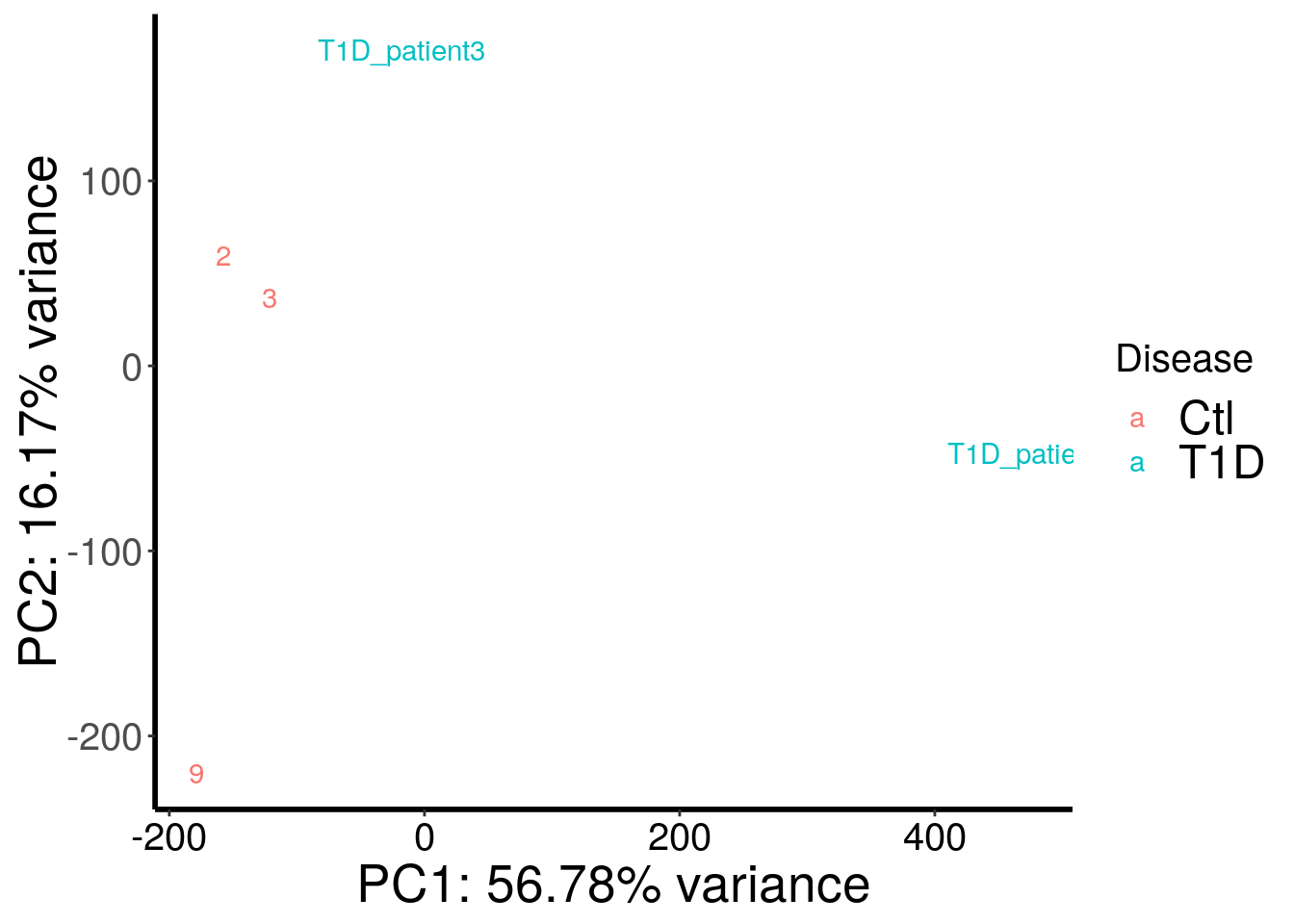
DM tests with RADAR
T1D_patient_RADAR <- diffIP_parallel(T1D_patient_RADAR, thread = 20)
T1D_patient_RADAR <- reportResult(T1D_patient_RADAR, cutoff = 0.05, threads = 20)

save(T1D_patient_RADAR, file = "~/Rohit_T1D/stim_Patient_islets/T1D_patient_RADAR.RData")
write.table(results(T1D_patient_RADAR), file = "~/Rohit_T1D/stim_Patient_islets/T1D_patient_diffPeaks_FDR0.05.xls", sep = "\t", row.names = FALSE, col.names = TRUE, quote = FALSE)
Differentially methylated m6A sites at FDR 5% threshold.
library(RADAR)
load("~/Rohit_T1D/stim_Patient_islets/T1D_patient_RADAR.RData")
DT::datatable( results(T1D_patient_RADAR) , rownames = FALSE )
There are 2076 reported differential loci at FDR < 0.05 and logFoldChange > 0.5.Distribution of differential m6A
DMG_result <- results(T1D_patient_RADAR)There are 2076 reported differential loci at FDR < 0.05 and logFoldChange > 0.5.ggplot(DMG_result, aes( x = logFC) )+geom_histogram(color="black", fill="dark gray",bins = 60)+xlab("Log fold change")+theme_bw() + ylab("Count")+ theme(panel.border = element_blank(), panel.grid.major = element_blank(),
panel.grid.minor = element_blank(), axis.line = element_line(colour = "black",size = 0.8),axis.ticks = element_line(colour = "black",size = 0.8),
axis.text = element_text(size = 20,colour = "black"),axis.text.y = element_text(angle = 0) ,axis.title=element_text(size=25,) )+scale_y_continuous(expand = c(0,0) )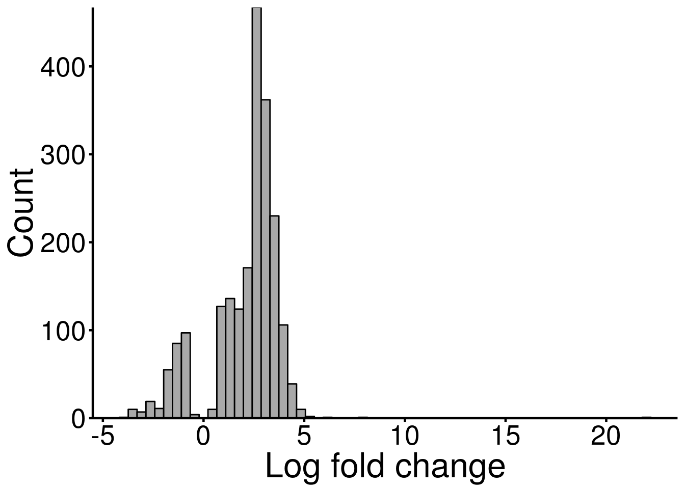
| Version | Author | Date |
|---|---|---|
| 41633ea | scottzijiezhang | 2020-09-09 |
There are some sparse large values up to ~ 20, so the x axis extended rightwards. For simplicity, I plot another histogram with cropped x-axis.
ggplot(DMG_result, aes( x = logFC)  )+geom_histogram(color="black", fill="dark gray",bins = 60)+xlab("Log fold change")+theme_bw() + ylab("Count")+ theme(panel.border = element_blank(), panel.grid.major = element_blank(),
                       panel.grid.minor = element_blank(), axis.line = element_line(colour = "black",size = 0.8),axis.ticks = element_line(colour = "black",size = 0.8),
axis.text = element_text(size = 20,colour = "black"),axis.text.y = element_text(angle = 0) ,axis.title=element_text(size=25,) )+scale_y_continuous(expand = c(0,0) )+scale_x_continuous(limits = c(-6,6))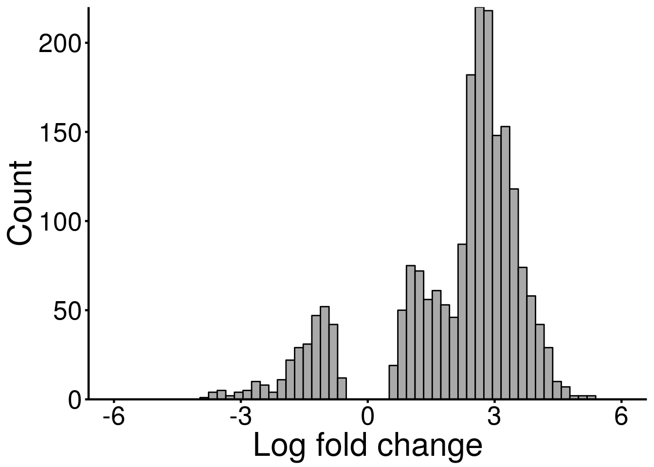
| Version | Author | Date |
|---|---|---|
| 41633ea | scottzijiezhang | 2020-09-09 |
ggplot(DMG_result, aes( x = logFC, y = -log10(p_value) )  )+geom_point()+xlab("Log fold change")+theme_bw() + ylab("- Log10(P-value)")+ theme(panel.border = element_blank(), panel.grid.major = element_blank(),
                       panel.grid.minor = element_blank(), axis.line = element_line(colour = "black",size = 0.8),axis.ticks = element_line(colour = "black",size = 0.8),
                       axis.text = element_text(size = 20,colour = "black"),axis.text.y = element_text(angle = 0) ,axis.title=element_text(size=25,) )+scale_y_continuous(expand = c(0,0), limits = c(0,14) )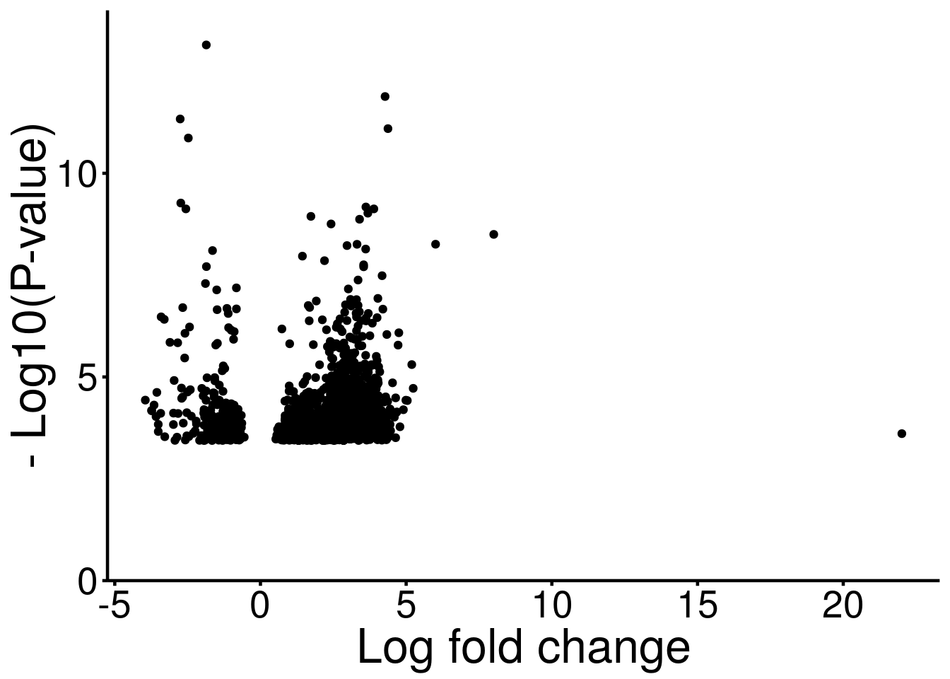
| Version | Author | Date |
|---|---|---|
| 41633ea | scottzijiezhang | 2020-09-09 |
Note this is not a standard volcano plot because only data points passing the threshold were plotted. This is just to visualize the P-values corresponding to the fold changes.
KEGG pathway analysis of DMG
library(clusterProfiler)
eg.PatDMG_DMG <- bitr( unique(results(T1D_patient_RADAR)$name), fromType="SYMBOL", toType="ENTREZID", OrgDb="org.Hs.eg.db")
There are 2076 reported differential loci at FDR < 0.05 and logFoldChange > 0.5.KEGG_PatDMG_DMG <- enrichKEGG(eg.PatDMG_DMG$ENTREZID,organism = "hsa",pAdjustMethod = "fdr", pvalueCutoff = 0.1,minGSSize = 3)No enriched termed found in KEGG pathway search. Plot coverage for selected genes
T1D_patient_RADAR <- PrepCoveragePlot(T1D_patient_RADAR)

plotGeneCov(T1D_patient_RADAR, geneName = "GAD2", libraryType = "opposite", center = mean, adjustExprLevel = TRUE )+ggtitle("GAD2")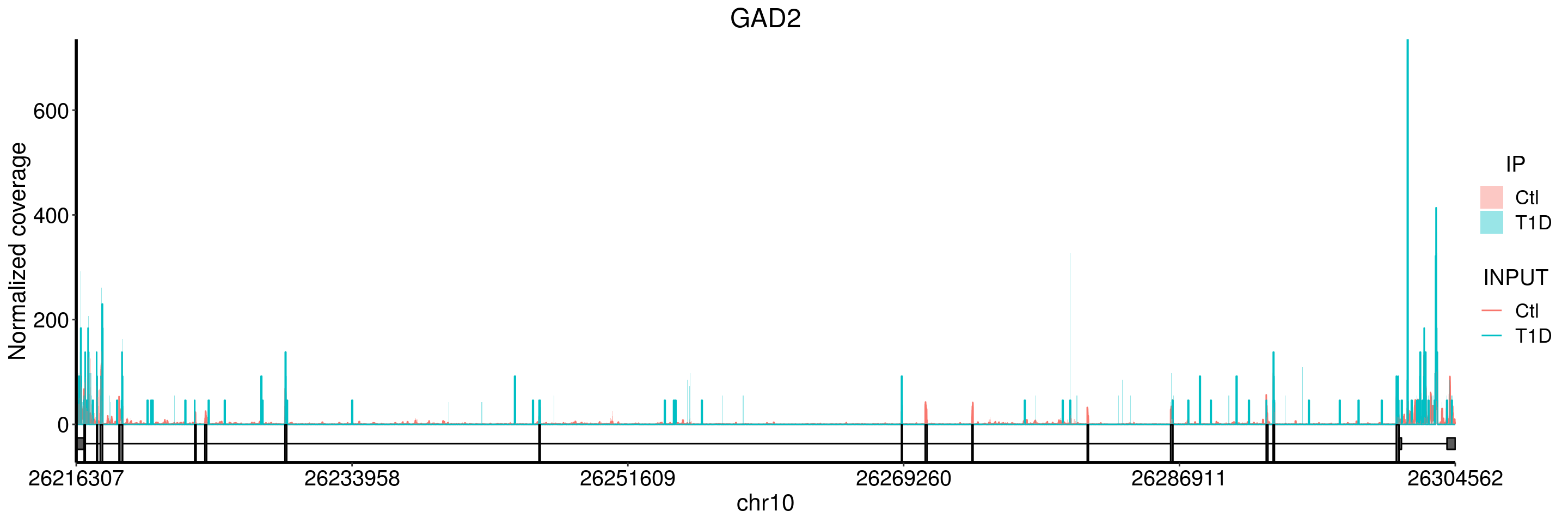
plotGeneCov(T1D_patient_RADAR, geneName = "GAD2", libraryType = "opposite", center = mean, ZoomIn = c(26216007, 26216656), adjustExprLevel = TRUE )+ggtitle("GAD2 zoom in")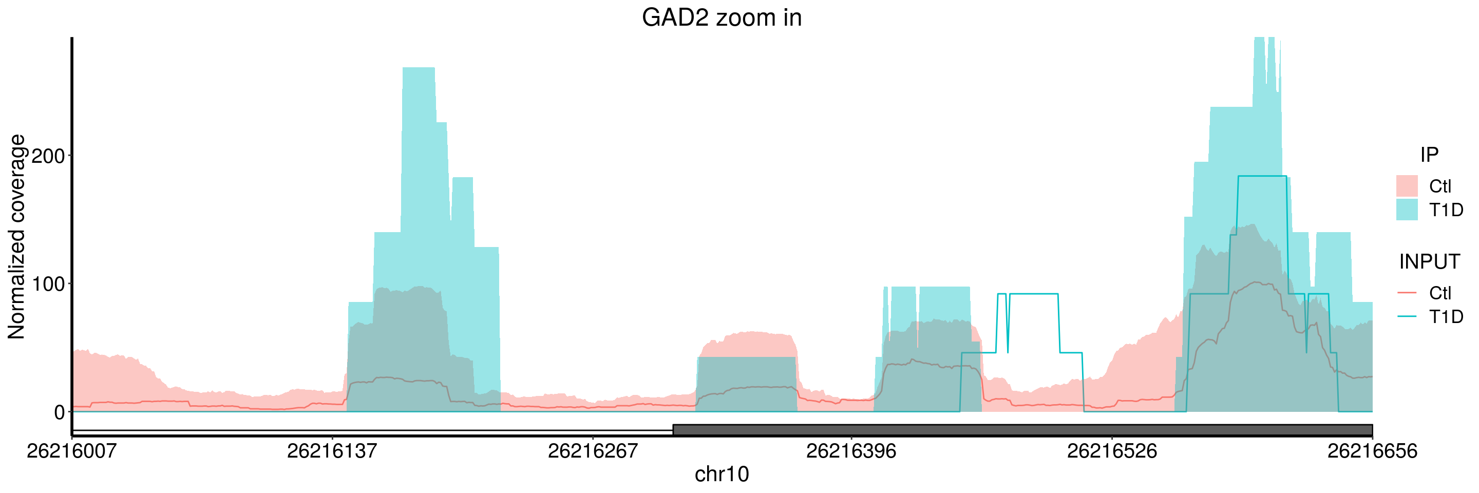 From the coverage plot, we can tell that the T1D samples have flat-shaped coverage, which indicates there many reads are likely identical and may result from PCR duplicates. Thus I would be cautious about the result of this gene, especially given our sample size are small here.
plotGeneCov(T1D_patient_RADAR, geneName = "HLA-A", libraryType = "opposite", center = mean, adjustExprLevel = TRUE )+ggtitle("HLA-A")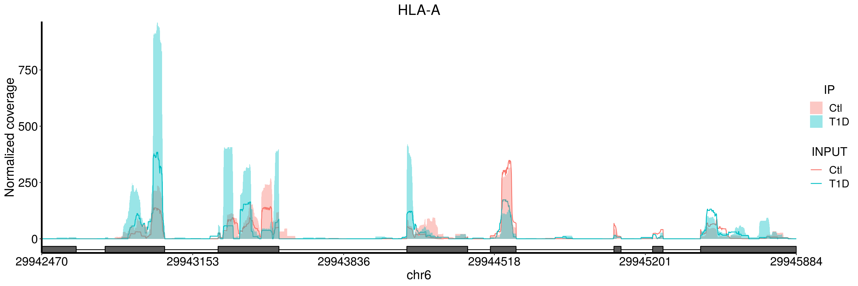
plotGeneCov(T1D_patient_RADAR, geneName = "HLA-B", libraryType = "opposite", center = mean, adjustExprLevel = TRUE )+ggtitle("HLA-B")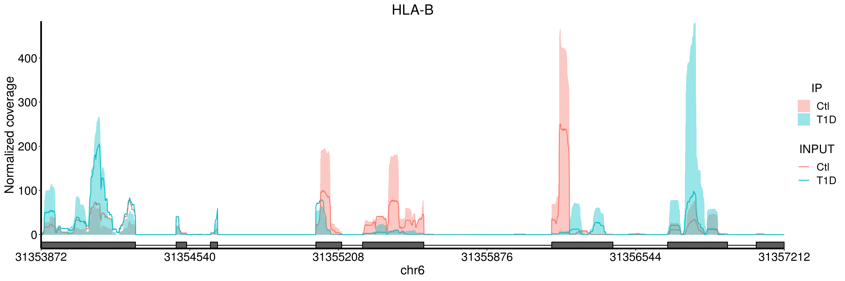
plotGeneCov(T1D_patient_RADAR, geneName = "HLA-B", libraryType = "opposite", center = mean,ZoomIn = c(31355280, 31355729), adjustExprLevel = TRUE )+ggtitle("HLA-B zoom in")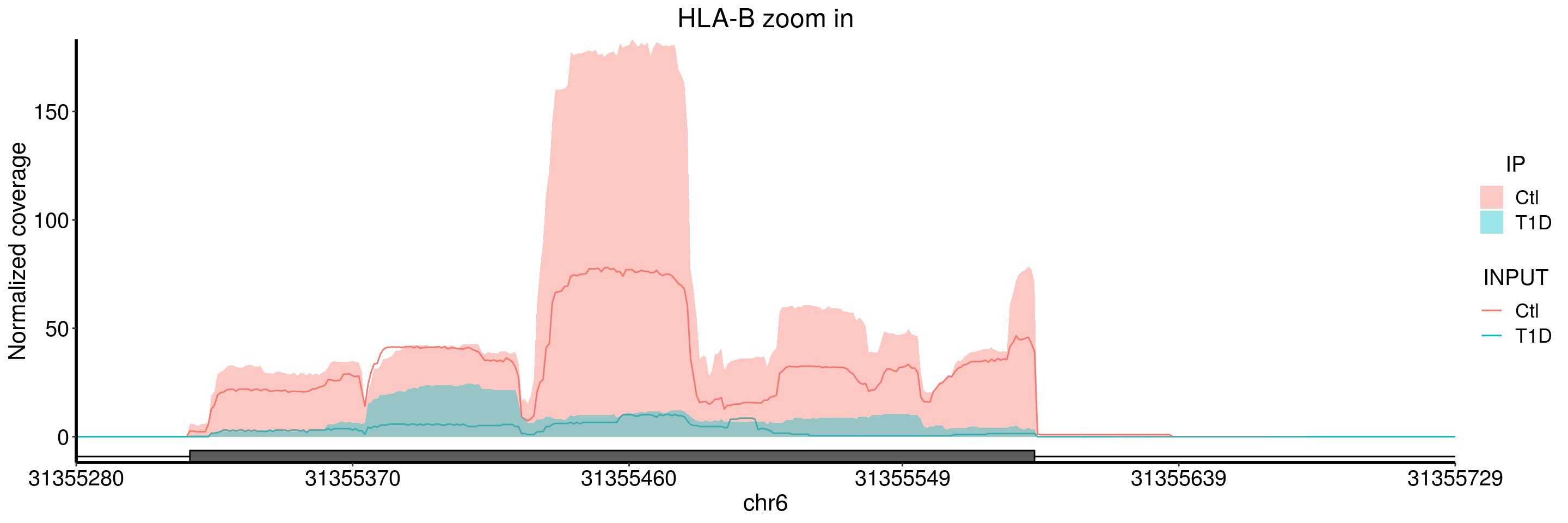
plotGeneCov(T1D_patient_RADAR, geneName = "PTPRN", libraryType = "opposite", center = mean, adjustExprLevel = TRUE )+ggtitle("PTPRN")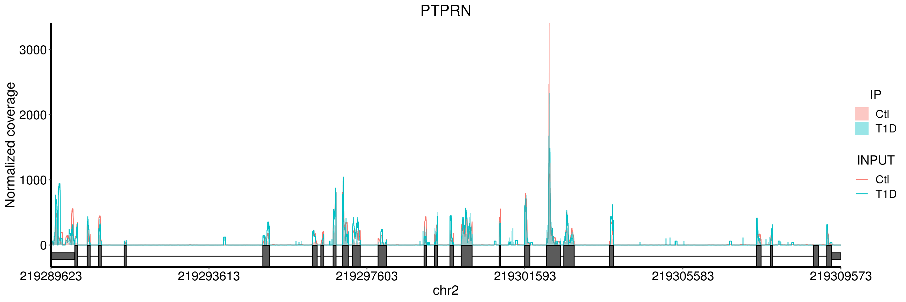
plotGeneCov(T1D_patient_RADAR, geneName = "PTPRN", libraryType = "opposite", center = mean,ZoomIn = c(219299509, 219299958), adjustExprLevel = TRUE )+ggtitle("PTPRN zoom in") This gene also show signs of bad data quality according to coverage of the T1D samples.
plotGeneCov(T1D_patient_RADAR, geneName = "PTPRN2", libraryType = "opposite", center = mean, adjustExprLevel = TRUE )+ggtitle("PTPRN2")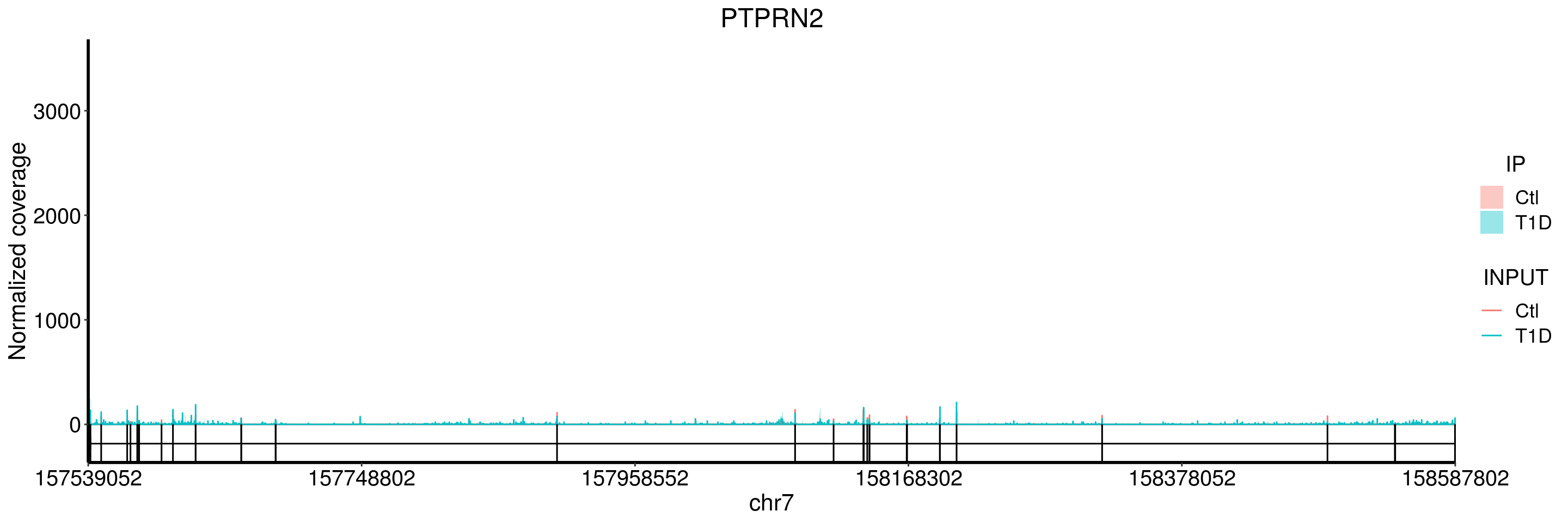
plotGeneCov(T1D_patient_RADAR, geneName = "PTPRN2", libraryType = "opposite", center = mean,ZoomIn = c(157540400, 157540849), adjustExprLevel = TRUE )+ggtitle("PTPRN2 zoom in")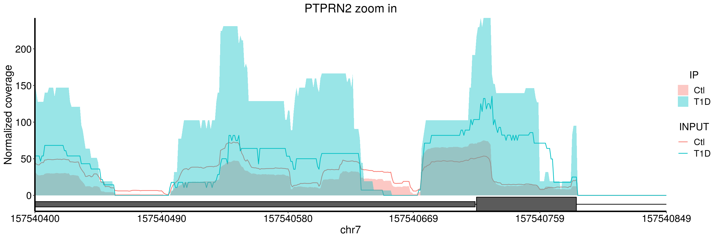
plotGeneCov(T1D_patient_RADAR, geneName = "INS", libraryType = "opposite", center = mean, adjustExprLevel = TRUE )+ggtitle("INS")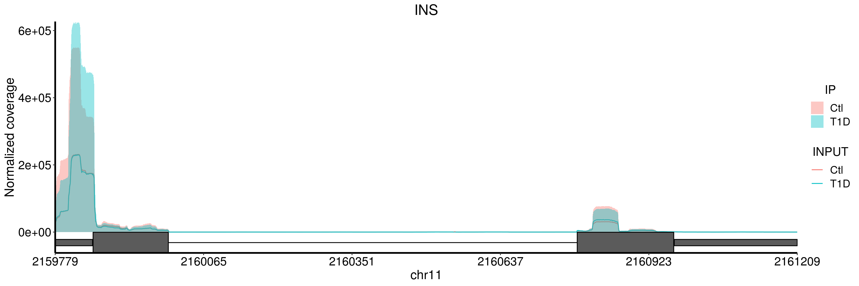
sessionInfo()R version 3.5.3 (2019-03-11)
Platform: x86_64-pc-linux-gnu (64-bit)
Running under: Ubuntu 17.10
Matrix products: default
BLAS: /usr/lib/x86_64-linux-gnu/openblas/libblas.so.3
LAPACK: /usr/lib/x86_64-linux-gnu/libopenblasp-r0.2.20.so
locale:
[1] LC_CTYPE=en_US.UTF-8 LC_NUMERIC=C
[3] LC_TIME=en_US.UTF-8 LC_COLLATE=en_US.UTF-8
[5] LC_MONETARY=en_US.UTF-8 LC_MESSAGES=en_US.UTF-8
[7] LC_PAPER=en_US.UTF-8 LC_NAME=C
[9] LC_ADDRESS=C LC_TELEPHONE=C
[11] LC_MEASUREMENT=en_US.UTF-8 LC_IDENTIFICATION=C
attached base packages:
[1] stats4 parallel stats graphics grDevices utils datasets
[8] methods base
other attached packages:
[1] org.Hs.eg.db_3.7.0 clusterProfiler_3.10.1
[3] RADAR_0.2.3 qvalue_2.14.1
[5] RcppArmadillo_0.9.400.2.0 Rcpp_1.0.1
[7] RColorBrewer_1.1-2 gplots_3.0.1.1
[9] doParallel_1.0.14 iterators_1.0.10
[11] foreach_1.4.4 ggplot2_3.1.1
[13] Rsamtools_1.34.1 Biostrings_2.50.2
[15] XVector_0.22.0 GenomicFeatures_1.34.8
[17] AnnotationDbi_1.44.0 Biobase_2.42.0
[19] GenomicRanges_1.34.0 GenomeInfoDb_1.18.2
[21] IRanges_2.16.0 S4Vectors_0.20.1
[23] BiocGenerics_0.28.0
loaded via a namespace (and not attached):
[1] backports_1.1.4 Hmisc_4.2-0
[3] fastmatch_1.1-0 workflowr_1.3.0
[5] plyr_1.8.4 igraph_1.2.4.1
[7] lazyeval_0.2.2 splines_3.5.3
[9] BiocParallel_1.16.6 crosstalk_1.0.0
[11] urltools_1.7.3 digest_0.6.18
[13] htmltools_0.3.6 GOSemSim_2.8.0
[15] viridis_0.5.1 GO.db_3.7.0
[17] gdata_2.18.0 magrittr_1.5
[19] checkmate_1.9.1 memoise_1.1.0
[21] cluster_2.0.7-1 annotate_1.60.1
[23] matrixStats_0.54.0 enrichplot_1.2.0
[25] prettyunits_1.0.2 colorspace_1.4-1
[27] blob_1.1.1 ggrepel_0.8.0
[29] xfun_0.6 dplyr_0.8.0.1
[31] crayon_1.3.4 RCurl_1.95-4.12
[33] jsonlite_1.6 genefilter_1.64.0
[35] survival_2.44-1.1 glue_1.3.1
[37] polyclip_1.10-0 gtable_0.3.0
[39] zlibbioc_1.28.0 UpSetR_1.3.3
[41] DelayedArray_0.8.0 scales_1.0.0
[43] DOSE_3.8.2 DBI_1.0.0
[45] viridisLite_0.3.0 xtable_1.8-4
[47] progress_1.2.0 htmlTable_1.13.1
[49] gridGraphics_0.3-0 foreign_0.8-71
[51] bit_1.1-14 europepmc_0.3
[53] Formula_1.2-3 DT_0.5.1
[55] htmlwidgets_1.3 httr_1.4.0
[57] fgsea_1.8.0 acepack_1.4.1
[59] pkgconfig_2.0.2 XML_3.98-1.19
[61] farver_1.1.0 nnet_7.3-12
[63] locfit_1.5-9.1 ggplotify_0.0.3
[65] tidyselect_0.2.5 labeling_0.3
[67] rlang_0.4.0 reshape2_1.4.3
[69] later_0.8.0 munsell_0.5.0
[71] tools_3.5.3 RSQLite_2.1.1
[73] ggridges_0.5.1 evaluate_0.13
[75] stringr_1.4.0 yaml_2.2.0
[77] knitr_1.22 bit64_0.9-7
[79] fs_1.3.0 caTools_1.17.1.2
[81] purrr_0.3.2 ggraph_1.0.2
[83] whisker_0.3-2 mime_0.6
[85] xml2_1.2.0 DO.db_2.9
[87] biomaRt_2.38.0 compiler_3.5.3
[89] rstudioapi_0.10 tibble_2.1.1
[91] tweenr_1.0.1 geneplotter_1.60.0
[93] stringi_1.4.3 lattice_0.20-38
[95] Matrix_1.2-17 pillar_1.3.1
[97] triebeard_0.3.0 data.table_1.12.2
[99] cowplot_0.9.4 bitops_1.0-6
[101] httpuv_1.5.1 rtracklayer_1.42.2
[103] R6_2.4.0 latticeExtra_0.6-28
[105] promises_1.0.1 KernSmooth_2.23-15
[107] gridExtra_2.3 codetools_0.2-16
[109] MASS_7.3-51.4 gtools_3.8.1
[111] assertthat_0.2.1 SummarizedExperiment_1.12.0
[113] DESeq2_1.22.2 rprojroot_1.3-2
[115] withr_2.1.2 GenomicAlignments_1.18.1
[117] GenomeInfoDbData_1.2.0 hms_0.4.2
[119] grid_3.5.3 rpart_4.1-13
[121] tidyr_0.8.3 rvcheck_0.1.3
[123] rmarkdown_1.12 git2r_0.25.2
[125] ggforce_0.2.2 shiny_1.3.2
[127] base64enc_0.1-3