Stim_human_islets
scottzijiezhang
2020-02-13
Last updated: 2020-08-26
Checks: 6 0
Knit directory: T1D_epitranscriptome/
This reproducible R Markdown analysis was created with workflowr (version 1.3.0). The Checks tab describes the reproducibility checks that were applied when the results were created. The Past versions tab lists the development history.
Great! Since the R Markdown file has been committed to the Git repository, you know the exact version of the code that produced these results.
Great job! The global environment was empty. Objects defined in the global environment can affect the analysis in your R Markdown file in unknown ways. For reproduciblity it’s best to always run the code in an empty environment.
The command set.seed(20190516) was run prior to running the code in the R Markdown file. Setting a seed ensures that any results that rely on randomness, e.g. subsampling or permutations, are reproducible.
Great job! Recording the operating system, R version, and package versions is critical for reproducibility.
Nice! There were no cached chunks for this analysis, so you can be confident that you successfully produced the results during this run.
Great! You are using Git for version control. Tracking code development and connecting the code version to the results is critical for reproducibility. The version displayed above was the version of the Git repository at the time these results were generated.
Note that you need to be careful to ensure that all relevant files for the analysis have been committed to Git prior to generating the results (you can use wflow_publish or wflow_git_commit). workflowr only checks the R Markdown file, but you know if there are other scripts or data files that it depends on. Below is the status of the Git repository when the results were generated:
Ignored files:
    Ignored:    .Rhistory
    Ignored:    analysis/.Rhistory

Untracked files:
    Untracked:  data/m6A.batch.out.RData
    Untracked:  data/m6A.batchGender.out.RData

Unstaged changes:
    Modified:   analysis/_site.yml
Note that any generated files, e.g. HTML, png, CSS, etc., are not included in this status report because it is ok for generated content to have uncommitted changes.
These are the previous versions of the R Markdown and HTML files. If you’ve configured a remote Git repository (see ?wflow_git_remote), click on the hyperlinks in the table below to view them.
| File | Version | Author | Date | Message |
|---|---|---|---|---|
| Rmd | 10e1965 | scottzijiezhang | 2020-08-26 | wflow_publish(c(“analysis/Human_betaCell_stim_QQQ.Rmd”, “analysis/NOD_mice_QQQ.Rmd”, “analysis/Stim_human_islets_RNAseq.Rmd”, |
| html | e150ef0 | scottzijiezhang | 2020-06-09 | Build site. |
| Rmd | a9eea4a | scottzijiezhang | 2020-06-09 | wflow_publish(“Stim_human_islets.Rmd”) |
| html | 891acee | scottzijiezhang | 2020-05-08 | Build site. |
| Rmd | 15f22e0 | scottzijiezhang | 2020-05-08 | wflow_publish(“Stim_human_islets.Rmd”) |
| html | 4879465 | scottzijiezhang | 2020-03-28 | Build site. |
| html | fc538cf | scottzijiezhang | 2020-03-09 | Build site. |
| html | cd6b7f8 | scottzijiezhang | 2020-02-27 | Build site. |
| Rmd | b421904 | scottzijiezhang | 2020-02-27 | wflow_publish(“Stim_human_islets.Rmd”) |
Introduction
Preprocessing and alignment
from <- list.files("~/Rohit_T1D/stim_Patient_islets/lane2/")
tmp <- gsub("CHe-SZ-48S-","",from)
tmp <- gsub("FC01-","",tmp)
tmp <- gsub("_001","",tmp)
tmp <- gsub("_S\\d+","",tmp)

repl_ID <- match( gsub("_R[0-9].fastq.gz","",tmp), paste0("T",1:88) )

to <- paste0(
  c(
  paste0( c( paste0( rep(1:5, rep(2,5) ), rep(c("","A"), 5) ),
        c("T1D_patient1","T1D_patient3"),
        paste0( rep(6:11, rep(2,6) ), rep(c("","A"), 6) )
        ), ".input"),
  paste0( c( paste0( rep(1:5, rep(2,5) ), rep(c("","A"), 5) ),
        c("T1D_patient1","T1D_patient3"),
        paste0( rep(6:11, rep(2,6) ), rep(c("","A"), 6) )
        ), ".m6A"),
  paste0( paste0( rep(12:21, rep(2,10) ), rep(c("","A"), 10) ),
        ".input"),
  paste0( paste0( rep(12:21, rep(2,10) ), rep(c("","A"), 10) ),
        ".m6A")
  )[repl_ID],
   gsub("T\\d+","",tmp)
  )

file.rename(paste0("~/Rohit_T1D/stim_Patient_islets/lane2/",from),paste0("~/Rohit_T1D/stim_Patient_islets/lane2/",to))

from <- list.files("~/Rohit_T1D/stim_Patient_islets/lane1/")
tmp <- gsub("CHe-SZ-48S-","",from)
tmp <- gsub("FC01-","",tmp)
tmp <- gsub("_001","",tmp)
tmp <- gsub("_L002","",tmp)
tmp <- gsub("_S\\d+","",tmp)

repl_ID <- match( gsub("_R[0-9].fastq.gz","",tmp), paste0("T",1:88) )

file.rename(paste0("~/Rohit_T1D/stim_Patient_islets/lane1/",from),paste0("~/Rohit_T1D/stim_Patient_islets/lane1/",to))
data_name <- c(
paste0( c( paste0( rep(1:5, rep(2,5) ), rep(c("","A"), 5) ),
c("T1D_patient1","T1D_patient3"),
paste0( rep(6:11, rep(2,6) ), rep(c("","A"), 6) )
), ".input"),
paste0( c( paste0( rep(1:5, rep(2,5) ), rep(c("","A"), 5) ),
c("T1D_patient1","T1D_patient3"),
paste0( rep(6:11, rep(2,6) ), rep(c("","A"), 6) )
), ".m6A"),
paste0( paste0( rep(12:21, rep(2,10) ), rep(c("","A"), 10) ),
".input"),
paste0( paste0( rep(12:21, rep(2,10) ), rep(c("","A"), 10) ),
".m6A")
)
filePath <- "~/Rohit_T1D/stim_Patient_islets/lane1/"
cutadapt <- paste0(" -a AGATCGGAAGAGCACACGTCTGAACTCCAGTCAC -A AGATCGGAAGAGCGTCGTGTAGGGAAAGAGTGTAGATCTCGGTGGTCGCCGTATCATT -o ",filePath,data_name,".trimmed.1.fastq.gz -p ",filePath,data_name,".trimmed.2.fastq.gz ",filePath,data_name,"_R1.fastq.gz ",filePath,data_name,"_R2.fastq.gz" )
for(i in cutadapt){
system2(command = "cutadapt", args = i , wait = F)
}
cutFirstThree <- paste0(" -u -3 -U 3 -m 20 -o ",filePath,data_name,".allTrimmed.1.fastq.gz -p ",filePath,data_name,".allTrimmed.2.fastq.gz ",filePath,data_name,".trimmed.1.fastq.gz ",filePath,data_name,".trimmed.2.fastq.gz" )
for(i in cutFirstThree){
system2(command = "cutadapt", args = i , wait = F)
}
file.remove( c(paste0(filePath,data_name,".trimmed.1.fastq.gz"),paste0(filePath,data_name,".trimmed.2.fastq.gz")) )
filePath <- "~/Rohit_T1D/stim_Patient_islets/lane2/"
cutadapt <- paste0(" -a AGATCGGAAGAGCACACGTCTGAACTCCAGTCAC -A AGATCGGAAGAGCGTCGTGTAGGGAAAGAGTGTAGATCTCGGTGGTCGCCGTATCATT -o ",filePath,data_name,".trimmed.1.fastq.gz -p ",filePath,data_name,".trimmed.2.fastq.gz ",filePath,data_name,"_R1.fastq.gz ",filePath,data_name,"_R2.fastq.gz" )
for(i in cutadapt){
system2(command = "cutadapt", args = i , wait = F)
}
cutFirstThree <- paste0(" -u -3 -U 3 -m 20 -o ",filePath,data_name,".allTrimmed.1.fastq.gz -p ",filePath,data_name,".allTrimmed.2.fastq.gz ",filePath,data_name,".trimmed.1.fastq.gz ",filePath,data_name,".trimmed.2.fastq.gz" )
for(i in cutFirstThree){
system2(command = "cutadapt", args = i , wait = F)
}
file.remove( c(paste0(filePath,data_name,".trimmed.1.fastq.gz"),paste0(filePath,data_name,".trimmed.2.fastq.gz")) )dir.create("~/Rohit_T1D/stim_Patient_islets/alignment_summary")
dir.create( out_dir <- "~/Rohit_T1D/stim_Patient_islets/bam_files/" )
dir.create( unalign <- "~/Rohit_T1D/stim_Patient_islets/unaligned_reads/" )
filePath1 <- "~/Rohit_T1D/stim_Patient_islets/lane1/"
filePath2 <- "~/Rohit_T1D/stim_Patient_islets/lane2/"
hisat_align <- paste0(" -x ~/Database/genome/hg38/hg38_UCSC --known-splicesite-infile ~/Database/genome/hg38/hisat2_splice_sites.txt -k 1 --un-conc-gz ",unalign,data_name,".unalign --summary-file ~/Rohit_T1D/stim_Patient_islets/alignment_summary/",data_name,".txt -p 20 --no-discordant -1 ",
filePath1,data_name,".allTrimmed.1.fastq.gz,",filePath2,data_name,".allTrimmed.1.fastq.gz -2 ",filePath1,data_name,".allTrimmed.2.fastq.gz,",filePath2,data_name,".allTrimmed.2.fastq.gz |samtools view -bS | samtools sort -o ", out_dir,data_name,".bam ")
for(i in hisat_align){
system2(command = "hisat2", args = i,wait = T )
}library(RADAR)
samplename <- c( paste0( rep(1:21, rep(2,21) ), rep(c("","A"), 21) ), c("T1D_patient1","T1D_patient3") )
allSampleRADAR <- countReads(samplenames = samplename,
gtf = "~/Database/genome/hg38/hg38_UCSC.gtf",
bamFolder = "~/Rohit_T1D/stim_Patient_islets/bam_files/",
outputDir = "~/Rohit_T1D/stim_Patient_islets/",
modification = "m6A",
binSize = 50,
paired = TRUE,
threads = 20
)
save(allSampleRADAR, file = "~/Rohit_T1D/stim_Patient_islets/allSample_RADAR.RData")Stimulated patient samples
load( "~/Rohit_T1D/stim_Patient_islets/allSample_RADAR.RData")

stim_patient_sample <- paste0( rep(1:15, rep(2,15) ), rep(c("","A"), 15) )

stim_patient_RADAR <- select(allSampleRADAR, stim_patient_sample)

stim_patient_RADAR <- normalizeLibrary(stim_patient_RADAR)
stim_patient_RADAR <- adjustExprLevel(stim_patient_RADAR)

variable(stim_patient_RADAR) <- data.frame(stim = rep(c("Ctl","Stim"), 15),
                                           gender = rep(c("F","M","M","M","M","F","M","M","M","M","F","F","M","M","M"),rep(2,15)),
                                           batch = c(rep("A",10),rep("B",12),rep("C",8)),
                                           age = rep(c(62,20,24,45,61,40,52,41,21,51,57,42,57,42,62),rep(2,15))
                                           )
stim_patient_RADAR <- filterBins(stim_patient_RADAR)
save(stim_patient_RADAR, file = "~/Rohit_T1D/stim_Patient_islets/stim_patient_RADAR.RData")
Check confounding factors
library(RADAR)
load( "~/Rohit_T1D/stim_Patient_islets/stim_patient_RADAR.RData")

plotPCAfromMatrix(stim_patient_RADAR@ip_adjExpr_filtered, variable(stim_patient_RADAR)$stim  )+scale_color_discrete(name = "Treatment")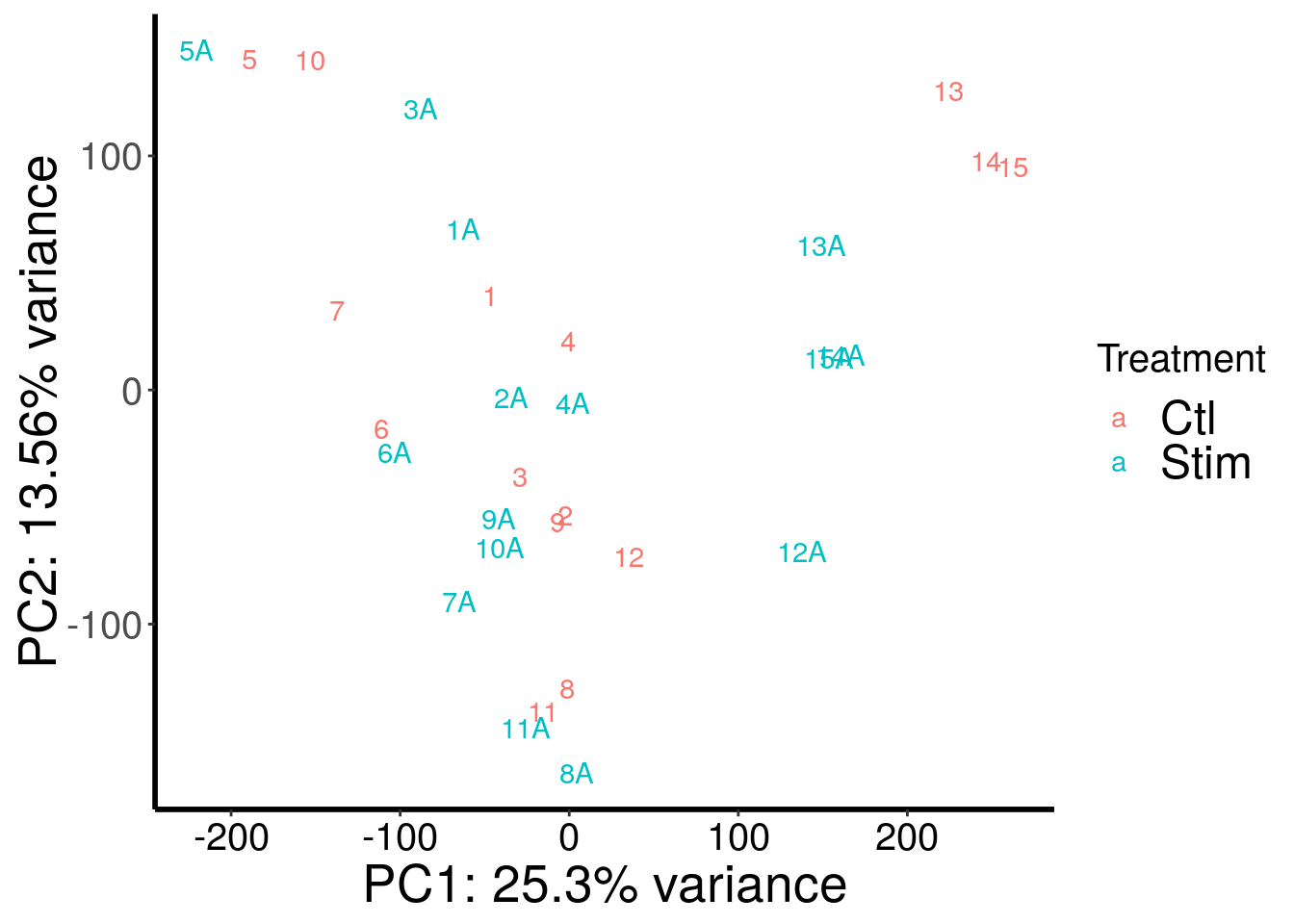
| Version | Author | Date |
|---|---|---|
| cd6b7f8 | scottzijiezhang | 2020-02-27 |
plotPCAfromMatrix(stim_patient_RADAR@ip_adjExpr_filtered, c(rep("A",10),rep("B",12),rep("C",8)) )+scale_color_discrete(name = "Batch")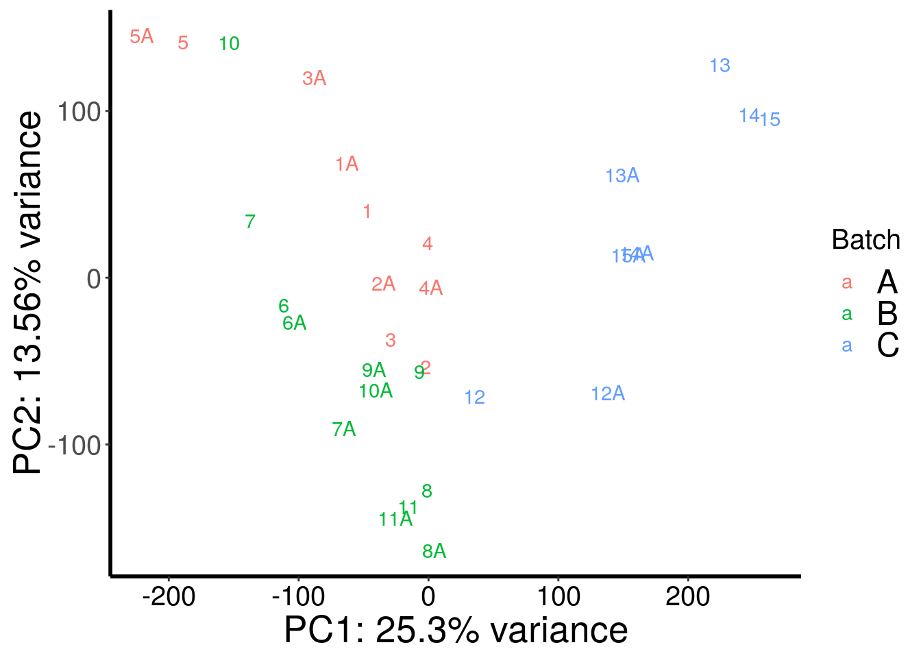
| Version | Author | Date |
|---|---|---|
| cd6b7f8 | scottzijiezhang | 2020-02-27 |
plotPCAfromMatrix(stim_patient_RADAR@ip_adjExpr_filtered, rep(c("F","M","M","M","M","F","M","M","M","M","F","F","M","M","M"),rep(2,15)) )+scale_color_discrete(name = "Gender")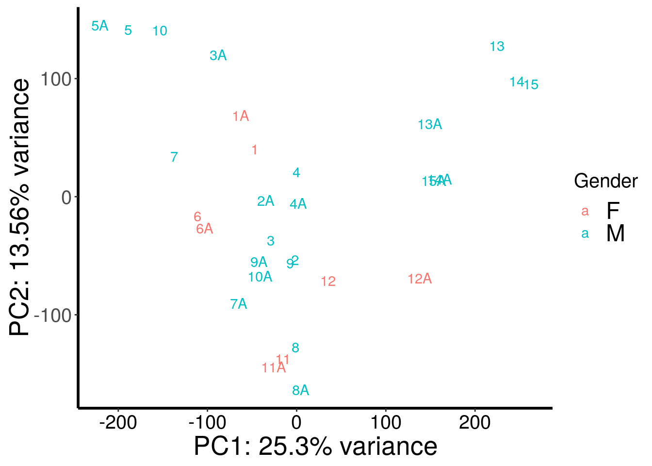
| Version | Author | Date |
|---|---|---|
| cd6b7f8 | scottzijiezhang | 2020-02-27 |
plotPCAfromMatrix(stim_patient_RADAR@ip_adjExpr_filtered, rep(c(62,20,24,45,61,40,52,41,21,51,57,42,57,42,62),rep(2,15)) )+scale_color_continuous(name = "Age")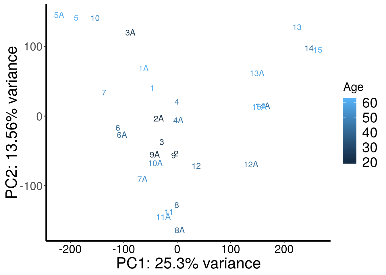
| Version | Author | Date |
|---|---|---|
| cd6b7f8 | scottzijiezhang | 2020-02-27 |
PCA analysis showed that m6A-IP batch explained a big proportion of variation.
Regress out batch and check the PCA
library(rafalib)
X2 <- as.fumeric( c(rep("A",10),rep("B",12),rep("A",8)) )-1 # batch as covariates
X3 <- as.fumeric( c(rep("A",10),rep("A",12),rep("C",8)) )-1 # batch as covariates

registerDoParallel(cores = 20)
m6A.cov.out <- foreach(i = 1:nrow( stim_patient_RADAR@ip_adjExpr_filtered ), .combine = rbind) %dopar% {
  Y = stim_patient_RADAR@ip_adjExpr_filtered[i,]
  resi <- residuals( lm(log(Y+1) ~ X2 + X3 ) )
  resi
}
rm(list=ls(name=foreach:::.foreachGlobals), pos=foreach:::.foreachGlobals)
rownames(m6A.cov.out) <- rownames(stim_patient_RADAR@ip_adjExpr_filtered)
save(m6A.cov.out, file = "~/Rohit_T1D/T1D_epitranscriptome/data/m6A.batch.out.RData")
load("~/Rohit_T1D/T1D_epitranscriptome/data/m6A.batch.out.RData")
RADAR::plotPCAfromMatrix(m6A.cov.out, c(rep("A",10),rep("B",12),rep("C",8)) , loglink = FALSE )+scale_color_discrete(name = "Batch")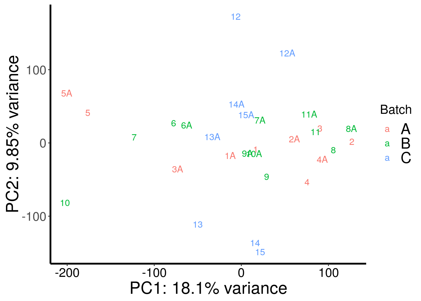
| Version | Author | Date |
|---|---|---|
| cd6b7f8 | scottzijiezhang | 2020-02-27 |
RADAR::plotPCAfromMatrix(m6A.cov.out, variable(stim_patient_RADAR)$stim , loglink = FALSE )+scale_color_discrete(name = "Treatment")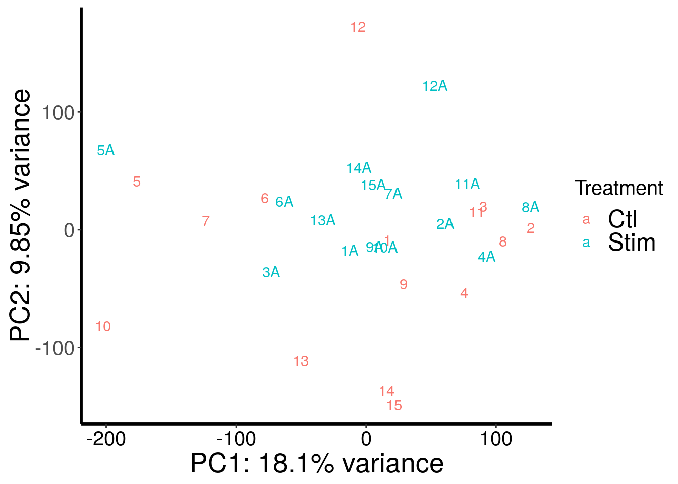
| Version | Author | Date |
|---|---|---|
| cd6b7f8 | scottzijiezhang | 2020-02-27 |
RADAR::plotPCAfromMatrix(m6A.cov.out, rep(c("F","M","M","M","M","F","M","M","M","M","F","F","M","M","M"),rep(2,15)) , loglink = FALSE )+scale_color_discrete(name = "Gender")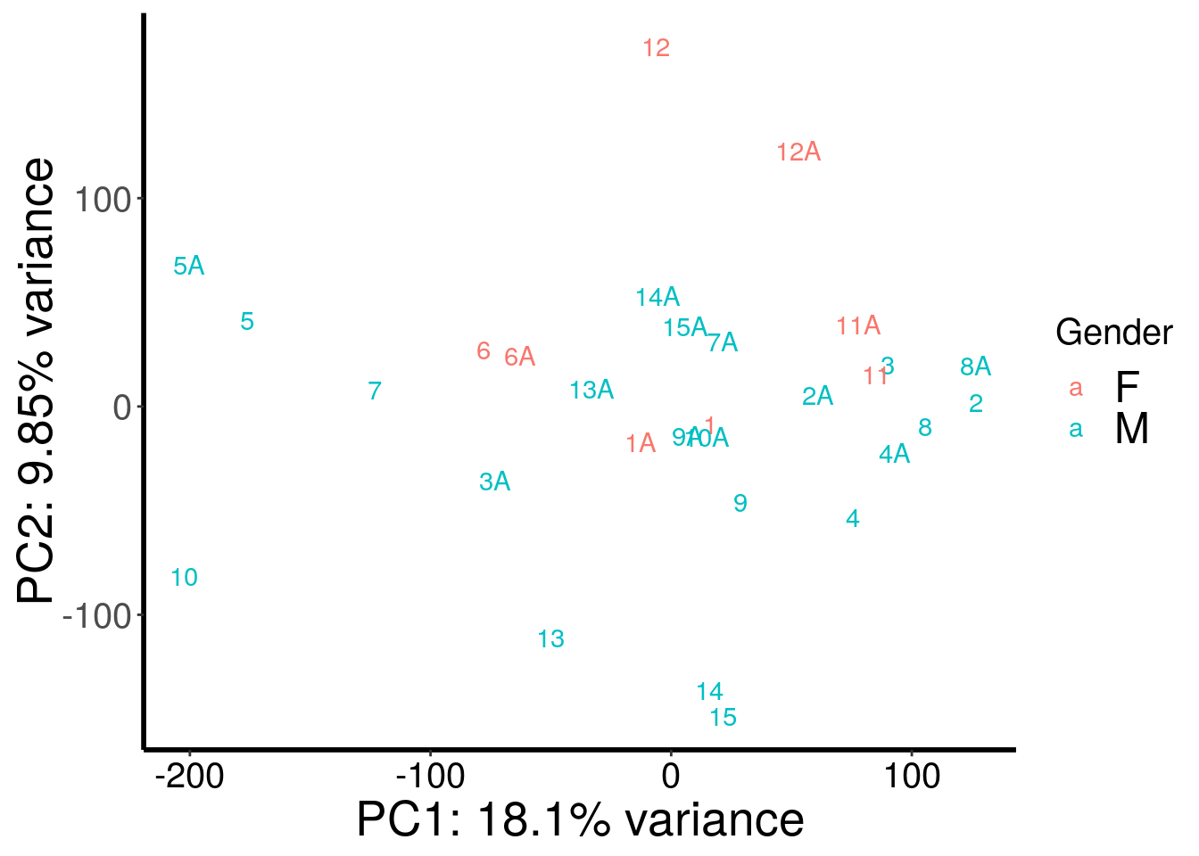
| Version | Author | Date |
|---|---|---|
| cd6b7f8 | scottzijiezhang | 2020-02-27 |
RADAR::plotPCAfromMatrix(m6A.cov.out, rep(c(62,20,24,45,61,40,52,41,21,51,57,42,57,42,62),rep(2,15)) , loglink = FALSE )+scale_color_continuous(name = "Age")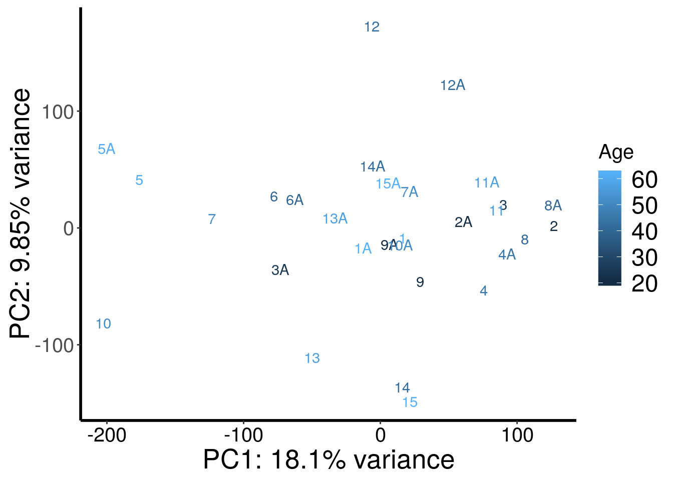
| Version | Author | Date |
|---|---|---|
| cd6b7f8 | scottzijiezhang | 2020-02-27 |
After regressing out batch, gender stand out as an confounding factor. Thus, we further regress out gender.
library(rafalib)
X2 <- as.fumeric( c(rep("A",10),rep("B",12),rep("A",8)) )-1 # batch as covariates
X3 <- as.fumeric( c(rep("A",10),rep("A",12),rep("C",8)) )-1 # batch as covariates
X4 <- as.fumeric( rep(c("F","M","M","M","M","F","M","M","M","M","F","F","M","M","M"),rep(2,15)) )-1 # gender as covariates

registerDoParallel(cores = 20)
m6A.batchGender.out <- foreach(i = 1:nrow( stim_patient_RADAR@ip_adjExpr_filtered ), .combine = rbind) %dopar% {
  Y = stim_patient_RADAR@ip_adjExpr_filtered[i,]
  resi <- residuals( lm(log(Y+1) ~ X2 + X3 + X4 ) )
  resi
}
rm(list=ls(name=foreach:::.foreachGlobals), pos=foreach:::.foreachGlobals)
rownames(m6A.batchGender.out) <- rownames(stim_patient_RADAR@ip_adjExpr_filtered)
save(m6A.batchGender.out, file = "~/Rohit_T1D/T1D_epitranscriptome/data/m6A.batchGender.out.RData")
load("~/Rohit_T1D/T1D_epitranscriptome/data/m6A.batchGender.out.RData")
RADAR::plotPCAfromMatrix(m6A.batchGender.out, variable(stim_patient_RADAR)$stim , loglink = FALSE )+scale_color_discrete(name = "Treatment")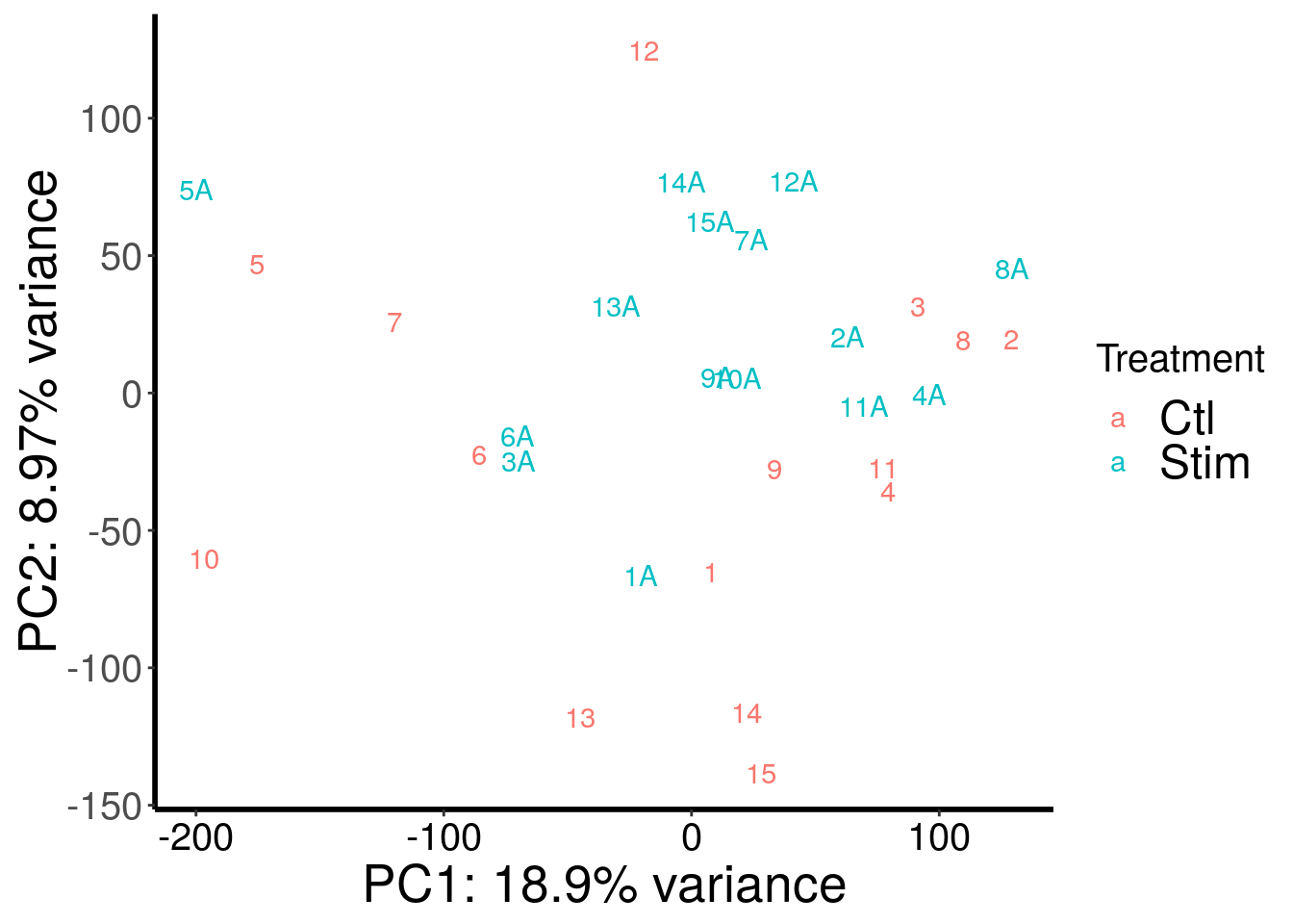
| Version | Author | Date |
|---|---|---|
| cd6b7f8 | scottzijiezhang | 2020-02-27 |
RADAR::plotPCAfromMatrix(m6A.batchGender.out, rep(c(62,20,24,45,61,40,52,41,21,51,57,42,57,42,62),rep(2,15)) , loglink = FALSE )+scale_color_continuous(name = "Age")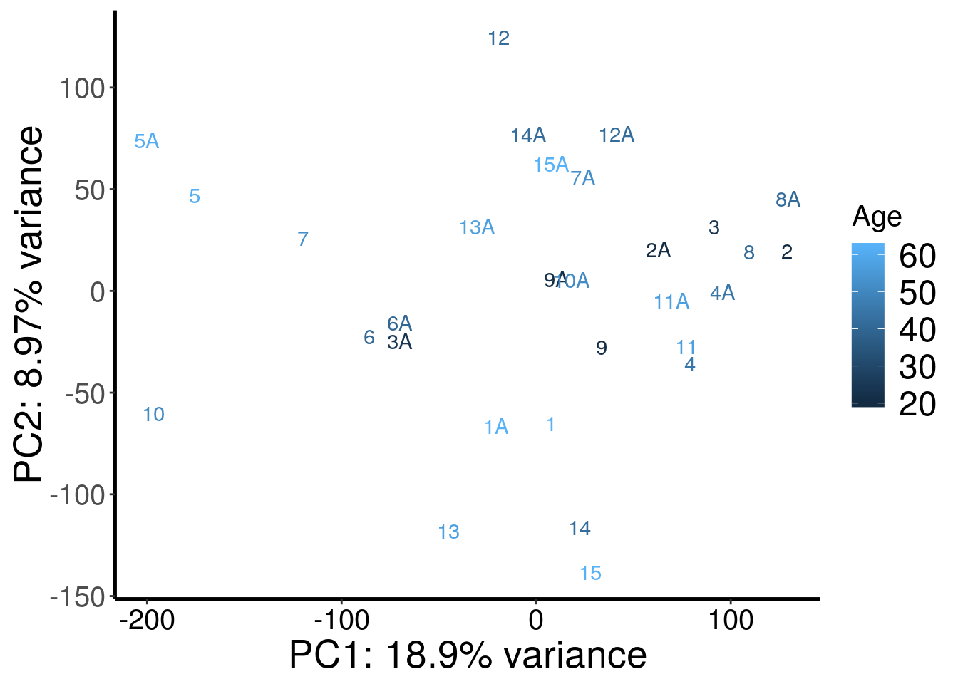
| Version | Author | Date |
|---|---|---|
| cd6b7f8 | scottzijiezhang | 2020-02-27 |
According to PCA, gender and batch are variables that explained significant proportion of variation. Thus, we include batch and gender as covariates in differential methylated test.
DM tests with RADAR
variable(stim_patient_RADAR) <- data.frame(stim = rep(c("Ctl","Stim"), 15),
                                           gender = as.fumeric( rep(c("F","M","M","M","M","F","M","M","M","M","F","F","M","M","M"),rep(2,15)) )-1 ,
                                           batch1 = as.fumeric( c(rep("A",10),rep("B",12),rep("A",8)) )-1 ,
                                           batch2 = as.fumeric( c(rep("A",10),rep("A",12),rep("C",8)) )-1
                                           )


stim_patient_RADAR <- diffIP_parallel(stim_patient_RADAR, thread = 20)
stim_patient_RADAR <- reportResult(stim_patient_RADAR, cutoff = 0.1, threads = 20)

save(stim_patient_RADAR, file = "~/Rohit_T1D/stim_Patient_islets/stim_patient_RADAR.RData")
write.table(results(stim_patient_RADAR), file = "~/Rohit_T1D/stim_Patient_islets/Stim_patient_diffPeaks_FDR0.1.xls", sep = "\t", row.names = FALSE, col.names = FALSE, quote = FALSE)
Differentially methylated m6A sites at FDR 10% threshold.
load("~/Rohit_T1D/stim_Patient_islets/stim_patient_RADAR.RData")
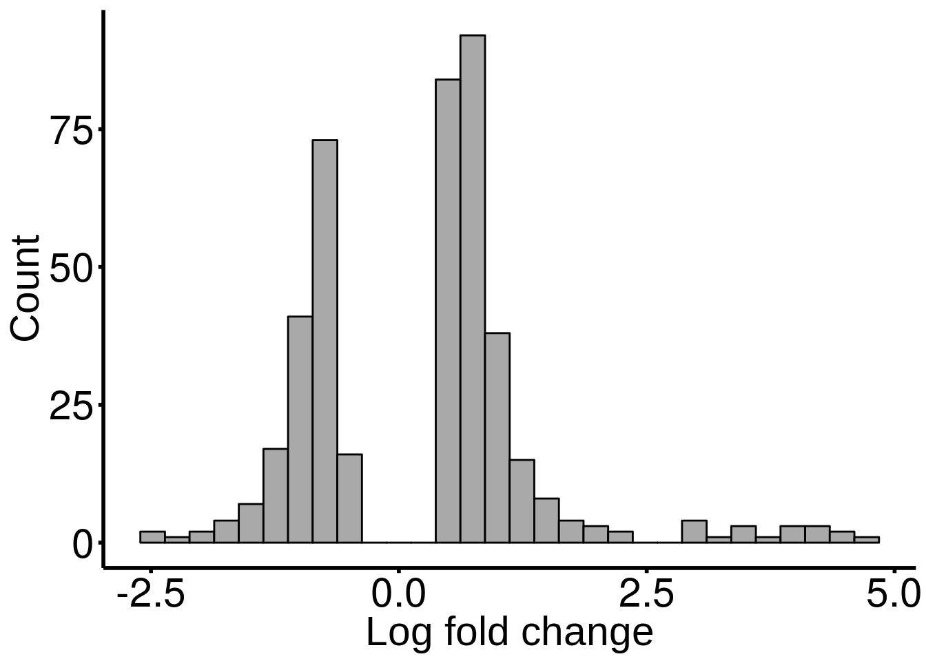
stim_patient_result <- results(stim_patient_RADAR)There are 427 reported differential loci at FDR < 0.1 and logFoldChange > 0.5.DT::datatable( stim_patient_result , rownames = FALSE )Distribution of log fold change of significant DM sites
ggplot(stim_patient_result ,aes( x = logFC ) )+geom_histogram(color="black", fill="dark gray",bins = 30)+xlab("Log fold change")+theme_bw() + ylab("Count")+ theme(panel.border = element_blank(), panel.grid.major = element_blank(),
                       panel.grid.minor = element_blank(), axis.line = element_line(colour = "black",size = 1),axis.ticks = element_line(colour = "black",size = 1), axis.text = element_text(size = 22,colour = "black"),axis.text.y = element_text(angle = 0) ,axis.title=element_text(size=22,family = "arial")
                       )
| Version | Author | Date |
|---|---|---|
| 891acee | scottzijiezhang | 2020-05-08 |
Spatial distribution of these DM sites
library(grid)
library(ggsci)
MeRIPtools::plotMetaGeneMulti( list("Hyper-methylated" = stim_patient_result[stim_patient_result$logFC>0,1:12], "Hypo-methylated" = stim_patient_result[stim_patient_result$logFC<0,1:12]), gtf = "~/Database/genome/hg38/hg38_UCSC.gtf" )
[1] "Converting BED12 to GRangesList"
[1] "It may take a few minutes"
[1] "Converting BED12 to GRangesList"
[1] "It may take a few minutes"
[1] "total 58259 transcripts extracted ..."
[1] "total 42543 transcripts left after ambiguity filter ..."
[1] "total 21293 mRNAs left after component length filter ..."
[1] "total 7986 ncRNAs left after ncRNA length filter ..."
[1] "Building Guitar Coordinates. It may take a few minutes ..."
[1] "Guitar Coordinates Built ..."
[1] "Using provided Guitar Coordinates"
[1] "resolving ambiguious features ..."
[1] "no figure saved ..."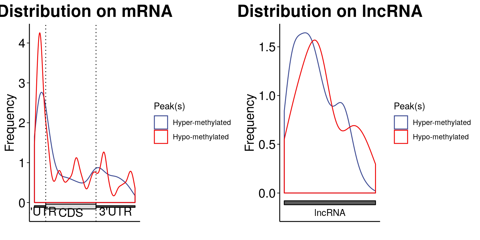
NOTE this function is a wrapper for R package "Guitar".
If you use the metaGene plot in publication, please cite the original reference:
Cui et al 2016 BioMed Research International
extendPeak <- function(peak, extension = 50){
peak_extend <- peak
peak_extend$start <- peak$start-extension
peak_extend$end <- peak$end+extension
peak_extend$blockSizes <- unlist( lapply( strsplit(as.character(peak$blockSizes),split = ",") , function(x){
tmp = as.numeric(x)
tmp[1] = tmp[1]+extension
tmp[length(tmp)] = tmp[length(tmp)]+extension
paste(as.character(tmp),collapse = ",")
} ) )
return(peak_extend)
}
## extend short peak for 50bp
stim_patient_DMpeak_extend <- extendPeak(stim_patient_result, extension = 15)
## analysis for RADAR detected signifiant bins
write.table(stim_patient_DMpeak_extend[,1:12], file = paste0("~/Rohit_T1D/stim_Patient_islets/Stim_patient_diffPeaks_FDR0.1.bed"),sep = "\t",row.names = F,col.names = F,quote = F)
system2(command = "bedtools", args = paste0("getfasta -fi ~/Database/genome/hg38/hg38_UCSC.fa -bed ~/Rohit_T1D/stim_Patient_islets/Stim_patient_diffPeaks_FDR0.1.bed -s -split > ~/Rohit_T1D/stim_Patient_islets/Stim_patient_diffPeaks_FDR0.1.fa ") )
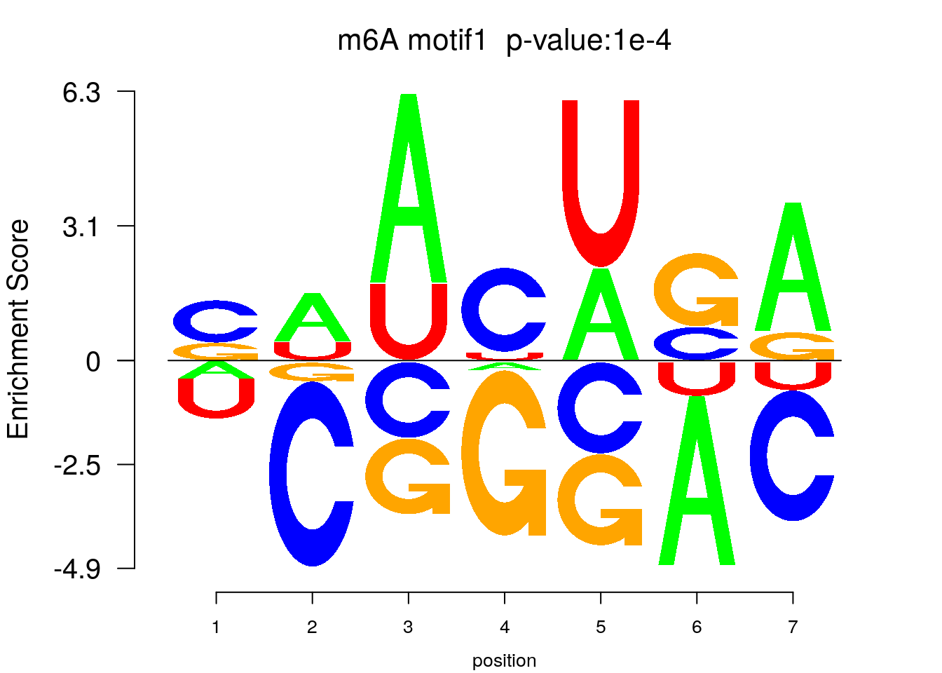
system2(command = "findMotifs.pl", args = paste0("~/Rohit_T1D/stim_Patient_islets/Stim_patient_diffPeaks_FDR0.1.fa fasta ~/Rohit_T1D/stim_Patient_islets/Stim_patient_diffPeaks_FDR0.1_Homer2 -fasta ~/Database/transcriptome/backgroud_peaks/hg38_200bp_randomPeak.fa -len 5,6 -rna -p 20 -S 5 -noknown"),wait = F )library(Logolas)
color_motif <- c( "orange", "blue", "red","green" )
for(i in 1:1){
pwm.m <- t( read.table(paste0("~/Rohit_T1D/stim_Patient_islets/Stim_patient_diffPeaks_FDR0.1_Homer2/homerResults/motif",i,".motif"), header = F, comment.char = ">",col.names = c("A","C","G","U")) )
motif_p <- sapply(1:1, function(x){
strsplit( as.character( read.table(paste0("~/Rohit_T1D/stim_Patient_islets/Stim_patient_diffPeaks_FDR0.1_Homer2/homerResults/motif",x,".motif"),comment.char = "", nrows = 1)[,12] ), split= ":")[[1]][4]
})
colnames(pwm.m) <- 1:ncol(pwm.m)
try(logomaker(pwm.m ,type = "EDLogo",colors = color_motif,color_type = "per_row" ,logo_control = list(pop_name = paste0("m6A motif",i," p-value:",motif_p[i])))
)
}
| Version | Author | Date |
|---|---|---|
| 891acee | scottzijiezhang | 2020-05-08 |
Note: the motif search result is not very good, but we can still see GAACU motif enriched among DM sites. One major problem here is that too few DM peaks are used for motif search and thus under powered.
Stimulated EndoC samples
load( "~/Rohit_T1D/stim_Patient_islets/allSample_RADAR.RData")

stim_EndoC_sample <- paste0( rep(16:21, rep(2,6) ), rep(c("","A"), 6) )

stim_EndoC_RADAR <- select(allSampleRADAR, stim_EndoC_sample)

stim_EndoC_RADAR <- normalizeLibrary(stim_EndoC_RADAR)
stim_EndoC_RADAR <- adjustExprLevel(stim_EndoC_RADAR)

variable(stim_EndoC_RADAR) <- data.frame(stim = rep(c("Ctl","Stim"), 6) )

stim_EndoC_RADAR <- filterBins(stim_EndoC_RADAR)
save(stim_EndoC_RADAR, file = "~/Rohit_T1D/stim_Patient_islets/stim_EndoC_RADAR.RData")
Check confounding factors
library(RADAR)
load( "~/Rohit_T1D/stim_Patient_islets/stim_EndoC_RADAR.RData")

plotPCAfromMatrix(stim_EndoC_RADAR@ip_adjExpr_filtered, variable(stim_EndoC_RADAR)$stim  )+scale_color_discrete(name = "Treatment")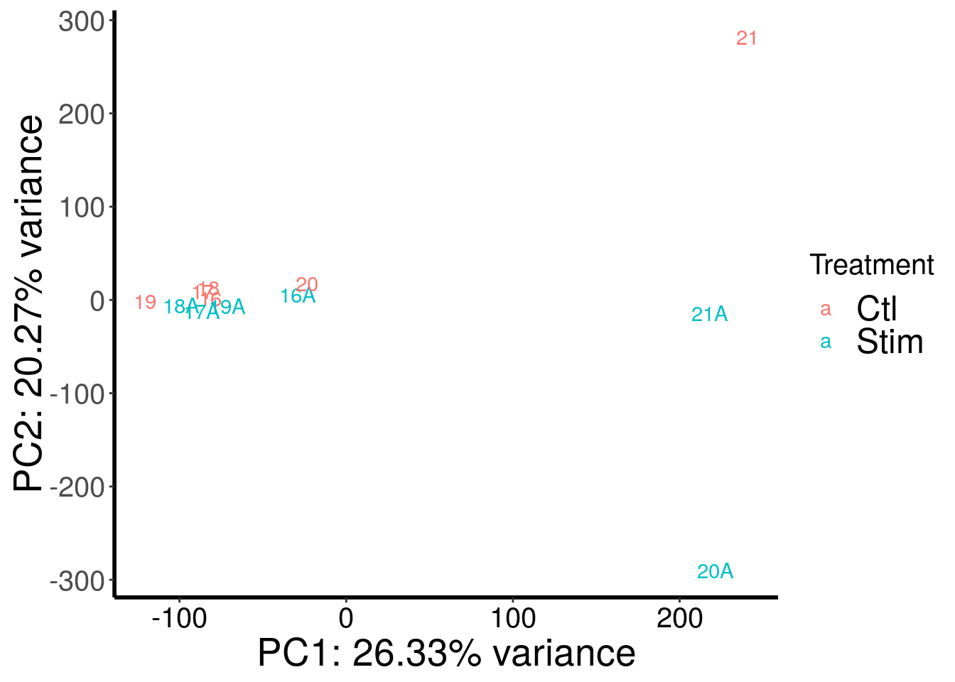
| Version | Author | Date |
|---|---|---|
| fc538cf | scottzijiezhang | 2020-03-09 |
Not sure what happened to sample 21 and 20A. PC1 seems to represent some technical variation.
DM test
stim_EndoC_RADAR <- diffIP_parallel(stim_EndoC_RADAR, thread = 20)
stim_EndoC_RADAR <- reportResult(stim_EndoC_RADAR, cutoff = 0.1, threads = 20)

save(stim_EndoC_RADAR, file = "~/Rohit_T1D/stim_Patient_islets/stim_EndoC_RADAR.RData")
write.table(results(stim_EndoC_RADAR), file = "~/Rohit_T1D/stim_Patient_islets/Stim_EndoC_diffPeaks_FDR0.1.xls", sep = "\t", row.names = FALSE, col.names = FALSE, quote = FALSE)
Differentially methylated m6A sites at FDR 10% threshold.
load("~/Rohit_T1D/stim_Patient_islets/stim_EndoC_RADAR.RData")
stim_EndoC_result <- results(stim_EndoC_RADAR)
There are 14 reported differential loci at FDR < 0.1 and logFoldChange > 0.5.DT::datatable( stim_EndoC_result , rownames = FALSE )Check m6A peaks in EP400, KDM2A, KMT2D and SMARCA2
EP400
nonStimPatientRadar <- RADAR::select(stim_patient_RADAR, samples = as.character(1:15) )Inferential test is not inherited because test result changes when samples are subsetted!
Please re-do test.plotGeneCov(stim_patient_RADAR, geneName = "EP400", libraryType = "opposite", adjustExprLevel = TRUE)+ggtitle("EP400")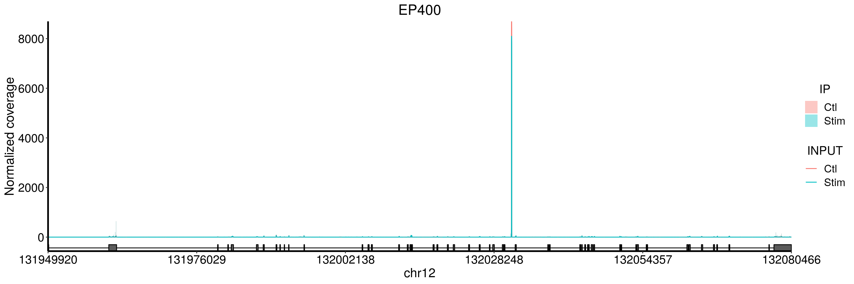
| Version | Author | Date |
|---|---|---|
| e150ef0 | scottzijiezhang | 2020-06-09 |
plotGeneCov(stim_patient_RADAR, geneName = "EP400", libraryType = "opposite", ZoomIn = c(131957920,131965920),adjustExprLevel = TRUE)+ggtitle("EP400 zoom in")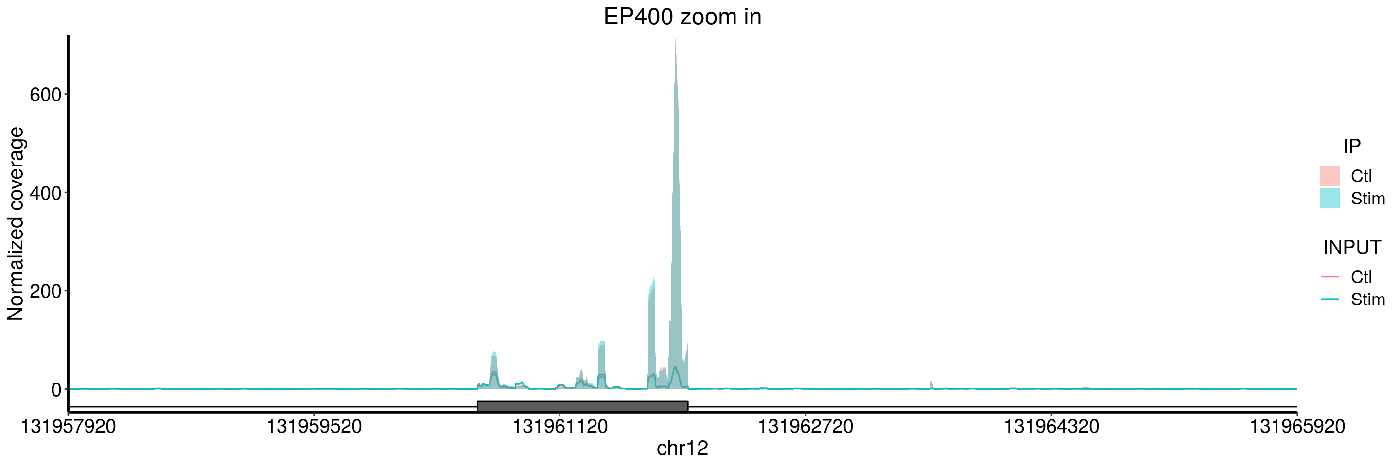
| Version | Author | Date |
|---|---|---|
| e150ef0 | scottzijiezhang | 2020-06-09 |
plotGeneCov(stim_patient_RADAR, geneName = "EP400", libraryType = "opposite", ZoomIn = c(132028248,132032248),adjustExprLevel = TRUE)+ggtitle("EP400 zoom in")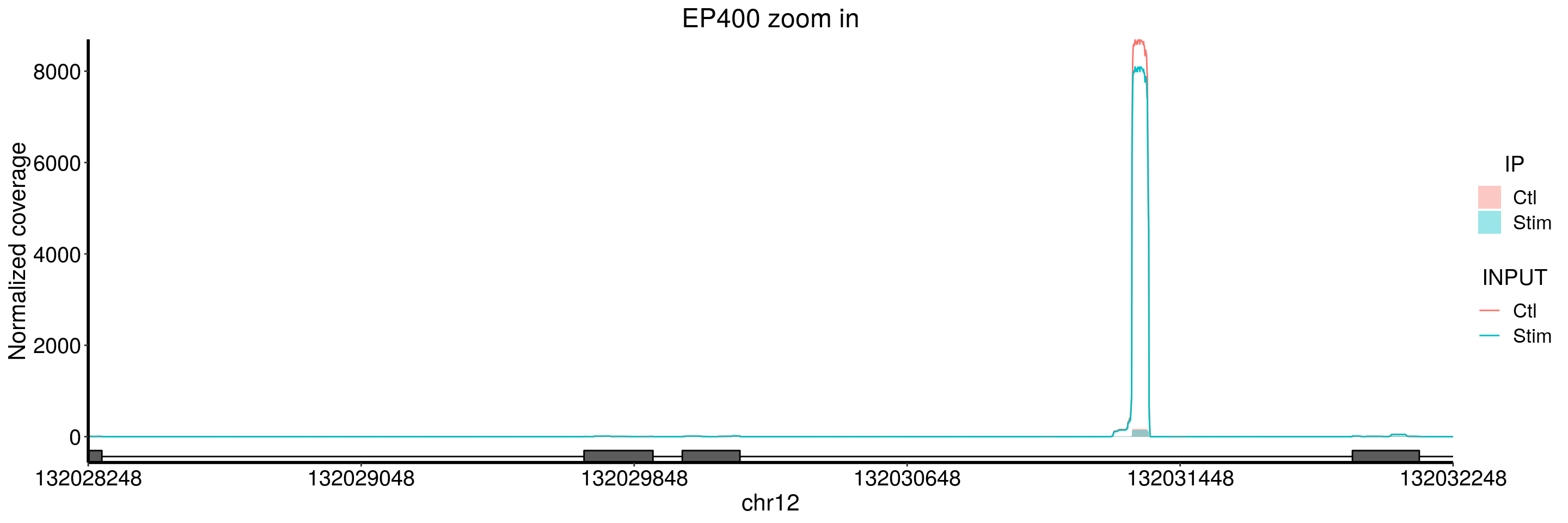
| Version | Author | Date |
|---|---|---|
| e150ef0 | scottzijiezhang | 2020-06-09 |
Note in the second zoom in, its just input but no IP coverage. This should correspond to the snoRNA as shown in the ALKBH5 CLIP peak.
KDM2A
plotGeneCov(stim_patient_RADAR, geneName = "KDM2A", libraryType = "opposite", adjustExprLevel = TRUE)+ggtitle("KDM2A")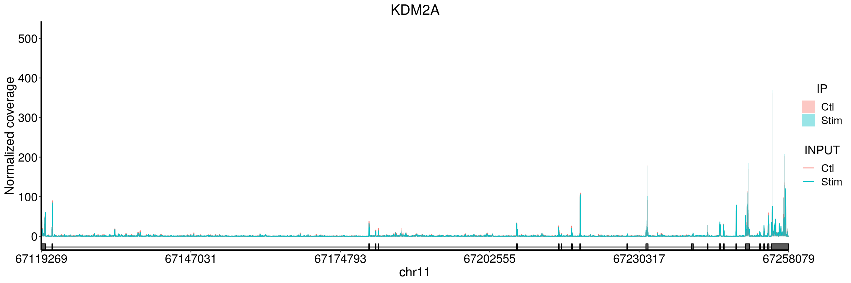
| Version | Author | Date |
|---|---|---|
| e150ef0 | scottzijiezhang | 2020-06-09 |
plotGeneCov(stim_patient_RADAR, geneName = "KDM2A", libraryType = "opposite", ZoomIn = c(67180393,67191000),adjustExprLevel = TRUE)+ggtitle("KDM2A zoom in")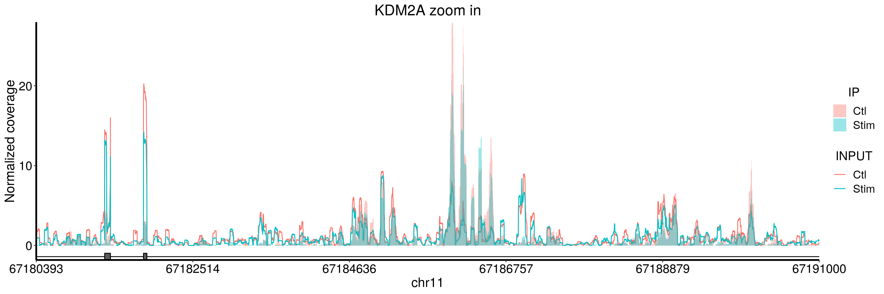
| Version | Author | Date |
|---|---|---|
| e150ef0 | scottzijiezhang | 2020-06-09 |
plotGeneCov(stim_patient_RADAR, geneName = "KDM2A", libraryType = "opposite", ZoomIn = c(67230317,67258079),adjustExprLevel = TRUE)+ggtitle("KDM2A zoom in")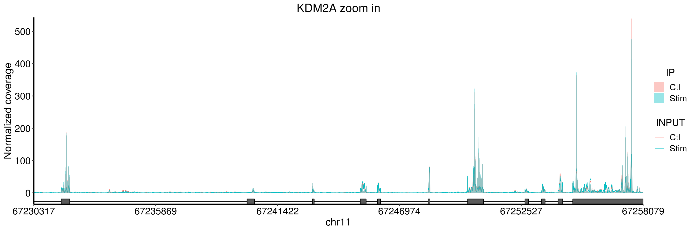
| Version | Author | Date |
|---|---|---|
| e150ef0 | scottzijiezhang | 2020-06-09 |
There is an intron methylation in KDM2A.
KMT2D
plotGeneCov(stim_patient_RADAR, geneName = "KMT2D", libraryType = "opposite", adjustExprLevel = TRUE)+ggtitle("KMT2D")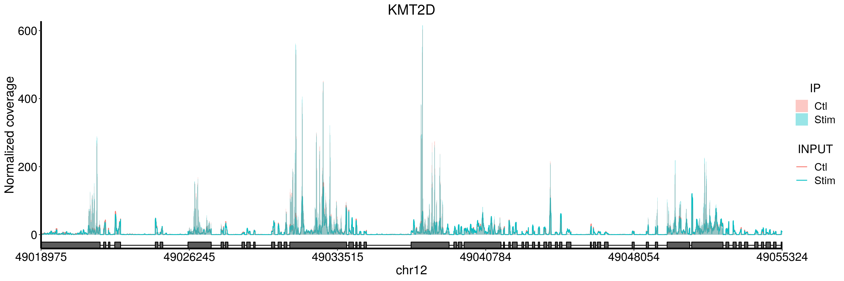
| Version | Author | Date |
|---|---|---|
| e150ef0 | scottzijiezhang | 2020-06-09 |
SMARCA2
plotGeneCov(stim_patient_RADAR, geneName = "SMARCA2", libraryType = "opposite", adjustExprLevel = TRUE)+ggtitle("SMARCA2")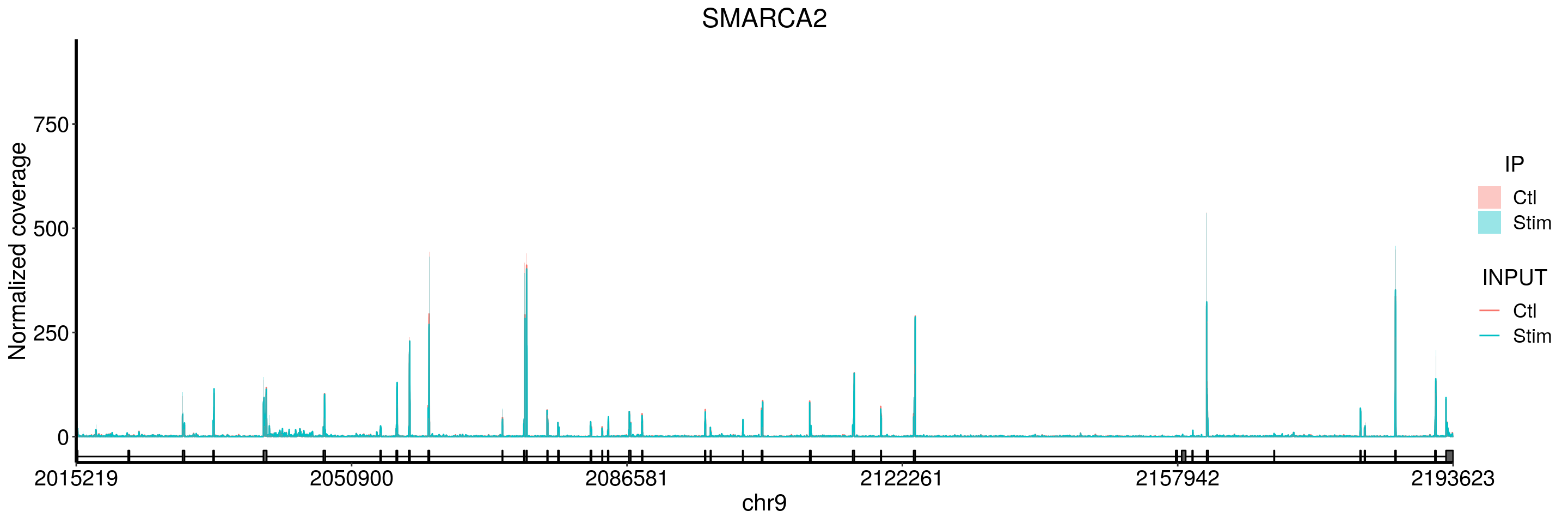
| Version | Author | Date |
|---|---|---|
| e150ef0 | scottzijiezhang | 2020-06-09 |
plotGeneCov(stim_patient_RADAR, geneName = "SMARCA2", libraryType = "opposite", ZoomIn = c(2015219,2050900),adjustExprLevel = TRUE)+ggtitle("SMARCA2 zoom in")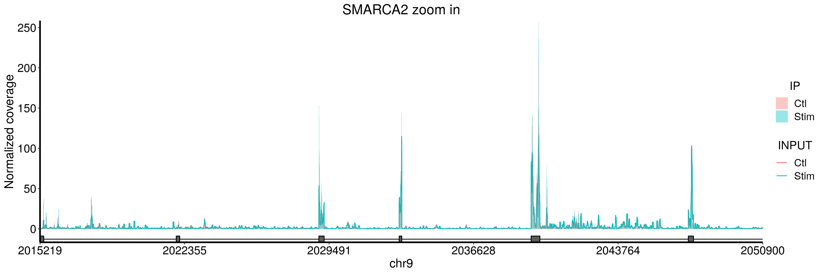
| Version | Author | Date |
|---|---|---|
| e150ef0 | scottzijiezhang | 2020-06-09 |
plotGeneCov(stim_patient_RADAR, geneName = "SMARCA2", libraryType = "opposite", ZoomIn = c(2157942,2193623),adjustExprLevel = TRUE)+ggtitle("SMARCA2 zoom in")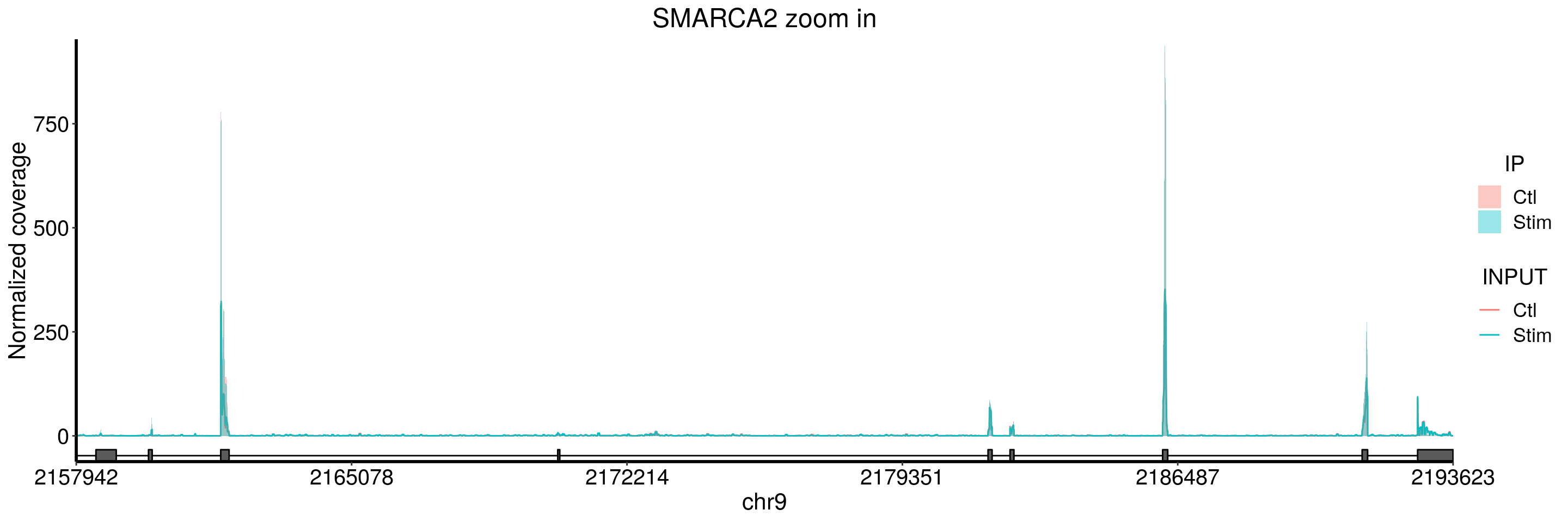
| Version | Author | Date |
|---|---|---|
| e150ef0 | scottzijiezhang | 2020-06-09 |
I don’t see peaks in SMARCA2 gene
sessionInfo()R version 3.5.3 (2019-03-11)
Platform: x86_64-pc-linux-gnu (64-bit)
Running under: Ubuntu 17.10
Matrix products: default
BLAS: /usr/lib/x86_64-linux-gnu/openblas/libblas.so.3
LAPACK: /usr/lib/x86_64-linux-gnu/libopenblasp-r0.2.20.so
locale:
[1] LC_CTYPE=en_US.UTF-8 LC_NUMERIC=C
[3] LC_TIME=en_US.UTF-8 LC_COLLATE=en_US.UTF-8
[5] LC_MONETARY=en_US.UTF-8 LC_MESSAGES=en_US.UTF-8
[7] LC_PAPER=en_US.UTF-8 LC_NAME=C
[9] LC_ADDRESS=C LC_TELEPHONE=C
[11] LC_MEASUREMENT=en_US.UTF-8 LC_IDENTIFICATION=C
attached base packages:
[1] grid stats4 parallel stats graphics grDevices utils
[8] datasets methods base
other attached packages:
[1] Logolas_1.6.0 ggsci_2.9
[3] RADAR_0.2.3 qvalue_2.14.1
[5] RcppArmadillo_0.9.400.2.0 Rcpp_1.0.1
[7] RColorBrewer_1.1-2 gplots_3.0.1.1
[9] doParallel_1.0.14 iterators_1.0.10
[11] foreach_1.4.4 ggplot2_3.1.1
[13] Rsamtools_1.34.1 Biostrings_2.50.2
[15] XVector_0.22.0 GenomicFeatures_1.34.8
[17] AnnotationDbi_1.44.0 Biobase_2.42.0
[19] GenomicRanges_1.34.0 GenomeInfoDb_1.18.2
[21] IRanges_2.16.0 S4Vectors_0.20.1
[23] BiocGenerics_0.28.0
loaded via a namespace (and not attached):
[1] backports_1.1.4 Hmisc_4.2-0
[3] workflowr_1.3.0 plyr_1.8.4
[5] lazyeval_0.2.2 splines_3.5.3
[7] gamlss_5.1-3 BiocParallel_1.16.6
[9] crosstalk_1.0.0 gridBase_0.4-7
[11] digest_0.6.18 htmltools_0.3.6
[13] SQUAREM_2017.10-1 gdata_2.18.0
[15] magrittr_1.5 checkmate_1.9.1
[17] memoise_1.1.0 BSgenome_1.50.0
[19] cluster_2.0.7-1 annotate_1.60.1
[21] matrixStats_0.54.0 prettyunits_1.0.2
[23] colorspace_1.4-1 blob_1.1.1
[25] exomePeak_2.16.0 gamlss.data_5.1-3
[27] xfun_0.6 dplyr_0.8.0.1
[29] crayon_1.3.4 RCurl_1.95-4.12
[31] jsonlite_1.6 genefilter_1.64.0
[33] survival_2.44-1.1 ape_5.3
[35] glue_1.3.1 gtable_0.3.0
[37] zlibbioc_1.28.0 DelayedArray_0.8.0
[39] scales_1.0.0 DBI_1.0.0
[41] viridisLite_0.3.0 xtable_1.8-4
[43] progress_1.2.0 htmlTable_1.13.1
[45] foreign_0.8-71 bit_1.1-14
[47] Formula_1.2-3 DT_0.5.1
[49] htmlwidgets_1.3 httr_1.4.0
[51] acepack_1.4.1 pkgconfig_2.0.2
[53] XML_3.98-1.19 nnet_7.3-12
[55] locfit_1.5-9.1 tidyselect_0.2.5
[57] labeling_0.3 rlang_0.4.0
[59] reshape2_1.4.3 later_0.8.0
[61] munsell_0.5.0 tools_3.5.3
[63] generics_0.0.2 RSQLite_2.1.1
[65] broom_0.5.2 evaluate_0.13
[67] stringr_1.4.0 yaml_2.2.0
[69] knitr_1.22 bit64_0.9-7
[71] fs_1.3.0 MeRIPtools_0.1.8
[73] caTools_1.17.1.2 purrr_0.3.2
[75] nlme_3.1-137 whisker_0.3-2
[77] mime_0.6 QNB_1.1.11
[79] biomaRt_2.38.0 compiler_3.5.3
[81] rstudioapi_0.10 Guitar_1.20.1
[83] tibble_2.1.1 geneplotter_1.60.0
[85] stringi_1.4.3 lattice_0.20-38
[87] Matrix_1.2-17 vegan_2.5-4
[89] permute_0.9-5 pillar_1.3.1
[91] data.table_1.12.2 bitops_1.0-6
[93] httpuv_1.5.1 rtracklayer_1.42.2
[95] R6_2.4.0 latticeExtra_0.6-28
[97] promises_1.0.1 vcfR_1.8.0
[99] KernSmooth_2.23-15 gridExtra_2.3
[101] codetools_0.2-16 MASS_7.3-51.4
[103] gtools_3.8.1 assertthat_0.2.1
[105] SummarizedExperiment_1.12.0 DESeq2_1.22.2
[107] rprojroot_1.3-2 withr_2.1.2
[109] pinfsc50_1.1.0 GenomicAlignments_1.18.1
[111] GenomeInfoDbData_1.2.0 mgcv_1.8-28
[113] hms_0.4.2 rpart_4.1-13
[115] tidyr_0.8.3 rmarkdown_1.12
[117] git2r_0.25.2 shiny_1.3.2
[119] gamlss.dist_5.1-3 base64enc_0.1-3