Human_betaCell_stim_QQQ
scottzijiezhang
2019-05-16
Last updated: 2020-08-27
Checks: 6 0
Knit directory: T1D_epitranscriptome/
This reproducible R Markdown analysis was created with workflowr (version 1.3.0). The Checks tab describes the reproducibility checks that were applied when the results were created. The Past versions tab lists the development history.
Great! Since the R Markdown file has been committed to the Git repository, you know the exact version of the code that produced these results.
Great job! The global environment was empty. Objects defined in the global environment can affect the analysis in your R Markdown file in unknown ways. For reproduciblity it’s best to always run the code in an empty environment.
The command set.seed(20190516) was run prior to running the code in the R Markdown file. Setting a seed ensures that any results that rely on randomness, e.g. subsampling or permutations, are reproducible.
Great job! Recording the operating system, R version, and package versions is critical for reproducibility.
Nice! There were no cached chunks for this analysis, so you can be confident that you successfully produced the results during this run.
Great! You are using Git for version control. Tracking code development and connecting the code version to the results is critical for reproducibility. The version displayed above was the version of the Git repository at the time these results were generated.
Note that you need to be careful to ensure that all relevant files for the analysis have been committed to Git prior to generating the results (you can use wflow_publish or wflow_git_commit). workflowr only checks the R Markdown file, but you know if there are other scripts or data files that it depends on. Below is the status of the Git repository when the results were generated:
Ignored files:
    Ignored:    .Rhistory
    Ignored:    analysis/.Rhistory

Untracked files:
    Untracked:  data/m6A.batch.out.RData
    Untracked:  data/m6A.batchGender.out.RData

Unstaged changes:
    Modified:   analysis/_site.yml
Note that any generated files, e.g. HTML, png, CSS, etc., are not included in this status report because it is ok for generated content to have uncommitted changes.
These are the previous versions of the R Markdown and HTML files. If you’ve configured a remote Git repository (see ?wflow_git_remote), click on the hyperlinks in the table below to view them.
| File | Version | Author | Date | Message |
|---|---|---|---|---|
| Rmd | 7f6b2ab | scottzijiezhang | 2020-08-27 | wflow_publish(“analysis/Human_betaCell_stim_QQQ.Rmd”) |
| html | 73c9f59 | scottzijiezhang | 2020-08-26 | Build site. |
| html | f707c22 | scottzijiezhang | 2020-08-15 | Build site. |
| Rmd | 043caa6 | scottzijiezhang | 2020-08-15 | wflow_publish(“Human_betaCell_stim_QQQ.Rmd”) |
| html | b4e8047 | scottzijiezhang | 2020-08-15 | Build site. |
| Rmd | 254da56 | scottzijiezhang | 2020-08-15 | wflow_publish(“Human_betaCell_stim_QQQ.Rmd”) |
| html | ba4b639 | scottzijiezhang | 2020-08-15 | Build site. |
| Rmd | 45f7148 | scottzijiezhang | 2020-08-15 | wflow_publish(“Human_betaCell_stim_QQQ.Rmd”) |
| html | ce13e24 | scottzijiezhang | 2020-08-13 | Build site. |
| Rmd | 23b8886 | scottzijiezhang | 2020-08-13 | wflow_publish(“Human_betaCell_stim_QQQ.Rmd”) |
| html | 605c6d1 | scottzijiezhang | 2019-05-20 | Build site. |
| Rmd | 066e941 | scottzijiezhang | 2019-05-20 | change y axis label |
| html | 2616200 | scottzijiezhang | 2019-05-20 | Build site. |
| Rmd | 0607fe2 | scottzijiezhang | 2019-05-20 | wflow_publish(“Human_betaCell_stim_QQQ.Rmd”) |
| html | 798a212 | scottzijiezhang | 2019-05-16 | Build site. |
| html | f4697b0 | scottzijiezhang | 2019-05-16 | Build site. |
| Rmd | 664897a | scottzijiezhang | 2019-05-16 | amend figures |
| html | 6c0f6d5 | scottzijiezhang | 2019-05-16 | Build site. |
| Rmd | 375441c | scottzijiezhang | 2019-05-16 | wflow_publish(“analysis/Human_betaCell_stim_QQQ.Rmd”) |
Introduction
Individual HP=19026-01
library(ggplot2)
library(ggpubr)
Loading required package: magrittr### quantify A
A_quant <- read.table("~/Rohit_T1D/Human_Islet_Stimu_QQQ/20190420_T1D_A.txt", sep = "\t", header = T, stringsAsFactors = F)[-c(1),c("Sample.Name","Sample.Type","Actual.Concentration","Area")]
for( i in 1:(nrow(A_quant)-1) ){ A_quant$group[i] <- (A_quant$Sample.Type[i]!=A_quant$Sample.Type[i+1] ) }
num_SampleGroup <- sum( A_quant$group)-1
Samples <- data.frame(start= (which(A_quant$group )+1)[1:num_SampleGroup], end = which(A_quant$group)[-c(1)])[seq(1,num_SampleGroup,2),]
result_A <- result_m6A <- result_G <- NULL
for(i in 1:nrow(Samples) ){
std_ID <- c( (Samples$start[i]-5):( Samples$start[i]-1), (Samples$end[i]+1):( Samples$end[i]+5))
A_quant_std <- dplyr::mutate_if(A_quant[std_ID,c("Actual.Concentration","Area")], is.character , as.numeric )
A_quant_tmp <-data.frame(Area = A_quant[Samples$start[i]:Samples$end[i],c("Area")])
fit <- lm(Actual.Concentration~Area, A_quant_std)
result_A <- rbind(result_A,cbind( "Name"= A_quant$Sample.Name[Samples$start[i]:Samples$end[i]], "A"= predict(fit, newdata = A_quant_tmp) ) )
}
### quantify G
G_quant <- read.table("~/Rohit_T1D/Human_Islet_Stimu_QQQ/20190420_T1D_G.txt", sep = "\t", header = T, stringsAsFactors = F)[-c(1),c("Sample.Name","Sample.Type","Actual.Concentration","Area")]
for(i in 1:nrow(Samples) ){
std_ID <- c( (Samples$start[i]-5):( Samples$start[i]-1), (Samples$end[i]+1):( Samples$end[i]+5))
G_quant_std <- dplyr::mutate_if(G_quant[std_ID,c("Actual.Concentration","Area")], is.character , as.numeric )
G_quant_tmp <-data.frame(Area = G_quant[Samples$start[i]:Samples$end[i],c("Area")])
fit <- lm(Actual.Concentration~Area, G_quant_std)
result_G <- rbind(result_G,cbind( "Name"= G_quant$Sample.Name[Samples$start[i]:Samples$end[i]], "G"= predict(fit, newdata = G_quant_tmp) ) )
}
### quantify m6A
m6A_quant <- read.table("~/Rohit_T1D/Human_Islet_Stimu_QQQ/20190420_T1D_m6A.txt", sep = "\t", header = T, stringsAsFactors = F)[-c(1),c("Sample.Name","Sample.Type","Actual.Concentration","Area")]
for(i in 1:nrow(Samples) ){
std_ID <- c( (Samples$start[i]-5):( Samples$start[i]-1), (Samples$end[i]+1):( Samples$end[i]+5))
m6A_quant_std <- dplyr::mutate_if(m6A_quant[std_ID,c("Actual.Concentration","Area")], is.character , as.numeric )
m6A_quant_tmp <-data.frame(Area = m6A_quant[Samples$start[i]:Samples$end[i],c("Area")])
fit <- lm(Actual.Concentration~Area, m6A_quant_std)
result_m6A <- rbind(result_m6A,cbind( "Name"= m6A_quant$Sample.Name[Samples$start[i]:Samples$end[i]], "m6A"= predict(fit, newdata = m6A_quant_tmp) ) )
}
result_batch1 <- data.frame( sampleName = rep( c("Basal", "Glucose 19mM","Insulin 10mM", "Palmitate 500uM","IL1b","INFa","INFg","TNFa","IL1b+INFa","IL1b+INFg"), 3) , A = as.numeric(result_A[,2]), G = as.numeric(result_G[,2]), m6A = as.numeric(result_m6A[,2]) )
result_batch1$m6AvsA <- result_batch1$m6A/result_batch1$A
result_batch1$m6AvsG <- result_batch1$m6A/result_batch1$G
DT::datatable(result_batch1, options = list(scrollX = TRUE, keys = TRUE, pageLength = 10),rownames = F)ggplot(result_batch1,aes( x = sampleName, y = m6AvsA))+geom_boxplot( )+ xlab("Samples") +ylab("m6A/A")+theme_bw()+theme(text = element_text(face = "bold", size = 20, color = "black"),axis.text = element_text(face = "bold", size = 16, color = "black"),axis.text.x = element_text(angle = 30,vjust = 0.7), axis.line = element_line(colour = "black", size = 0.75))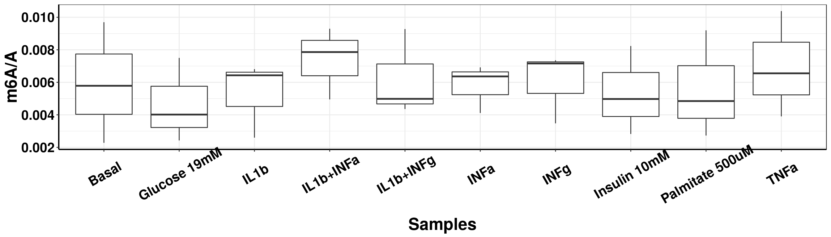
| Version | Author | Date |
|---|---|---|
| 6c0f6d5 | scottzijiezhang | 2019-05-16 |
ggplot(result_batch1)+geom_boxplot(aes( x = sampleName, y = m6AvsG) )+ xlab("Samples") +ylab("m6A/G") +theme_bw()+theme(text = element_text(face = "bold", size = 20, color = "black"),axis.text = element_text(face = "bold", size = 16, color = "black"),axis.text.x = element_text(angle = 30,vjust = 0.7), axis.line = element_line(colour = "black", size = 0.75))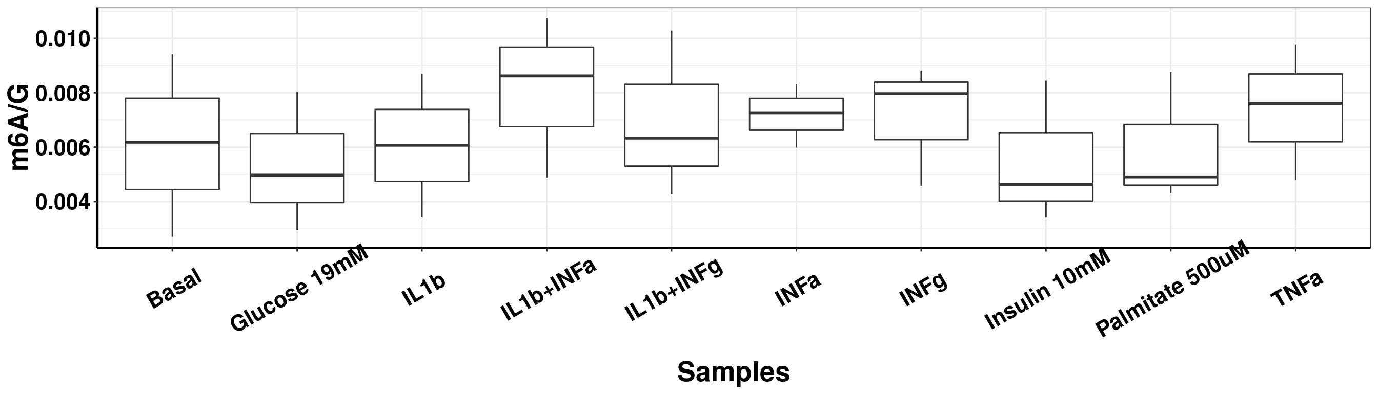
| Version | Author | Date |
|---|---|---|
| 6c0f6d5 | scottzijiezhang | 2019-05-16 |
### Individual HP=19030-01
library(ggplot2)
library(ggpubr)

### quantify A
A_quant <- read.table("~/Rohit_T1D/Human_Islet_Stimu_QQQ/20190515_T1D_A.txt", sep = "\t", header = T, stringsAsFactors = F)[-c(1),c("Sample.Name","Sample.Type","Actual.Concentration","Area")]

for( i in 1:(nrow(A_quant)-1) ){ A_quant$group[i] <- (A_quant$Sample.Type[i]!=A_quant$Sample.Type[i+1] ) }

num_SampleGroup <- sum( A_quant$group)-1

Samples <- data.frame(start= (which(A_quant$group )+1)[1:num_SampleGroup], end = which(A_quant$group)[-c(1)])[seq(1,num_SampleGroup,2),]

result_A <- result_m6A <- result_G <- result_m1A <- NULL
for(i in 1:nrow(Samples) ){
  std_ID <- c( (Samples$start[i]-5):( Samples$start[i]-1), (Samples$end[i]+1):( Samples$end[i]+5))
  A_quant_std <- dplyr::mutate_if(A_quant[std_ID,c("Actual.Concentration","Area")], is.character , as.numeric )
  A_quant_tmp <-data.frame(Area = A_quant[Samples$start[i]:Samples$end[i],c("Area")])
  fit <- lm(Actual.Concentration~Area, A_quant_std)
  result_A <- rbind(result_A,cbind( "Name"= A_quant$Sample.Name[Samples$start[i]:Samples$end[i]], "A"=  predict(fit, newdata = A_quant_tmp) ) )
}

### quantify G
G_quant <- read.table("~/Rohit_T1D/Human_Islet_Stimu_QQQ/20190515_T1D_G.txt", sep = "\t", header = T, stringsAsFactors = F)[-c(1),c("Sample.Name","Sample.Type","Actual.Concentration","Area")]

for(i in 1:nrow(Samples) ){
  std_ID <- c( (Samples$start[i]-5):( Samples$start[i]-1), (Samples$end[i]+1):( Samples$end[i]+5))
  G_quant_std <- dplyr::mutate_if(G_quant[std_ID,c("Actual.Concentration","Area")], is.character , as.numeric )
  G_quant_tmp <-data.frame(Area = G_quant[Samples$start[i]:Samples$end[i],c("Area")])
  fit <- lm(Actual.Concentration~Area, G_quant_std)
  result_G <- rbind(result_G,cbind( "Name"= G_quant$Sample.Name[Samples$start[i]:Samples$end[i]], "G"=  predict(fit, newdata = G_quant_tmp) ) )
}

### quantify m6A
m6A_quant <- read.table("~/Rohit_T1D/Human_Islet_Stimu_QQQ/20190515_T1D_m6A.txt", sep = "\t", header = T, stringsAsFactors = F)[-c(1),c("Sample.Name","Sample.Type","Actual.Concentration","Area")]

for(i in 1:nrow(Samples) ){
  std_ID <- c( (Samples$start[i]-5):( Samples$start[i]-1), (Samples$end[i]+1):( Samples$end[i]+5))
  m6A_quant_std <- dplyr::mutate_if(m6A_quant[std_ID,c("Actual.Concentration","Area")], is.character , as.numeric )
  m6A_quant_tmp <-data.frame(Area = m6A_quant[Samples$start[i]:Samples$end[i],c("Area")])
  fit <- lm(Actual.Concentration~Area, m6A_quant_std)
  result_m6A <- rbind(result_m6A,cbind( "Name"= m6A_quant$Sample.Name[Samples$start[i]:Samples$end[i]], "m6A"=  predict(fit, newdata = m6A_quant_tmp) ) )
}

### quantify m1A
m1A_quant <- read.table("~/Rohit_T1D/Human_Islet_Stimu_QQQ/20190515_T1D_m1A.txt", sep = "\t", header = T, stringsAsFactors = F)[-c(1),c("Sample.Name","Sample.Type","Actual.Concentration","Area")]

for(i in 1:nrow(Samples) ){
  std_ID <- c( (Samples$start[i]-5):( Samples$start[i]-1), (Samples$end[i]+1):( Samples$end[i]+5))
  m1A_quant_std <- dplyr::mutate_if(m1A_quant[std_ID,c("Actual.Concentration","Area")], is.character , as.numeric )
  m1A_quant_tmp <-data.frame(Area = m1A_quant[Samples$start[i]:Samples$end[i],c("Area")])
  fit <- lm(Actual.Concentration~Area, m1A_quant_std)
  result_m1A <- rbind(result_m1A,cbind( "Name"= m1A_quant$Sample.Name[Samples$start[i]:Samples$end[i]], "m1A"=  predict(fit, newdata = m1A_quant_tmp) ) )
}


result_batch2 <- data.frame( sampleName = rep( c("Basal", "Glucose 19mM","Insulin 10mM", "Palmitate 500uM","IL1b","INFa","INFg","TNFa","IL1b+INFa","IL1b+INFg"), 3) , A = as.numeric(result_A[,2]), G = as.numeric(result_G[,2]), m6A = as.numeric(result_m6A[,2]), m1A =  as.numeric(result_m1A[,2]) )
result_batch2$m6AvsA <- result_batch2$m6A/result_batch2$A
result_batch2$m6AvsG <- result_batch2$m6A/result_batch2$G
result_batch2$m1AvsA <- result_batch2$m1A/result_batch2$A
result_batch2$m1AvsG <- result_batch2$m1A/result_batch2$G

DT::datatable(result_batch2, options = list(scrollX = TRUE, keys = TRUE, pageLength = 10),rownames = F)
result_batch2_m6A_melt <- data.frame(sampleName = rep(result_batch2$sampleName,2), m6A = c(result_batch2$m6AvsA,result_batch2$m6AvsG), compareTo = c(rep("A",nrow(result_batch2) ),rep("G",nrow(result_batch2))) )
ggplot(result_batch2_m6A_melt,aes( x = sampleName, y = m6A, color = compareTo))+geom_boxplot( )+ xlab("Samples") +ylab("m6A/(A or G)")+theme_bw()+theme(text = element_text(face = "bold", size = 20, color = "black"),axis.text = element_text(face = "bold", size = 16, color = "black"),axis.text.x = element_text(angle = 30,vjust = 0.7), axis.line = element_line(colour = "black", size = 0.75))+geom_abline(intercept = mean(result_batch2$m6AvsA[result_batch2$sampleName=="Basal"]), slope = 0, lty = "dashed", colour ="#F8766D" )+geom_abline(intercept = mean(result_batch2$m6AvsG[result_batch2$sampleName=="Basal"]), slope = 0, lty = "dashed", colour ="#00BFC4" )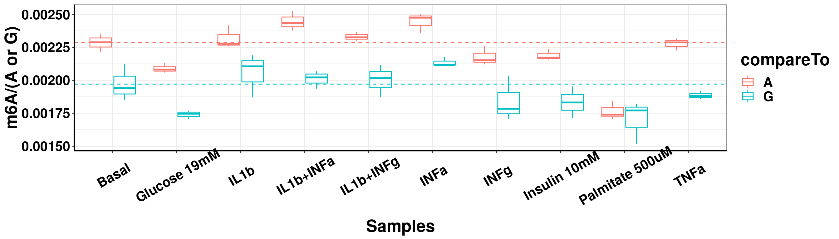
result_batch2_m1A_melt <- data.frame(sampleName = rep(result_batch2$sampleName,2), m1A = c(result_batch2$m1AvsA,result_batch2$m1AvsG), compareTo = c(rep("A",nrow(result_batch2) ),rep("G",nrow(result_batch2))) )
ggplot(result_batch2_m1A_melt,aes( x = sampleName, y = m1A, colour = compareTo))+geom_boxplot( )+ xlab("Samples") +ylab("m1A/(A or G)")+theme_bw()+theme(text = element_text(face = "bold", size = 20, color = "black"),axis.text = element_text(face = "bold", size = 16, color = "black"),axis.text.x = element_text(angle = 30,vjust = 0.7), axis.line = element_line(colour = "black", size = 0.75))+geom_abline(intercept = mean(result_batch2$m1AvsA[result_batch2$sampleName=="Basal"]), slope = 0, lty = "dashed", colour ="#F8766D"  )+geom_abline(intercept = mean(result_batch2$m1AvsG[result_batch2$sampleName=="Basal"]), slope = 0, lty = "dashed", colour ="#00BFC4"  )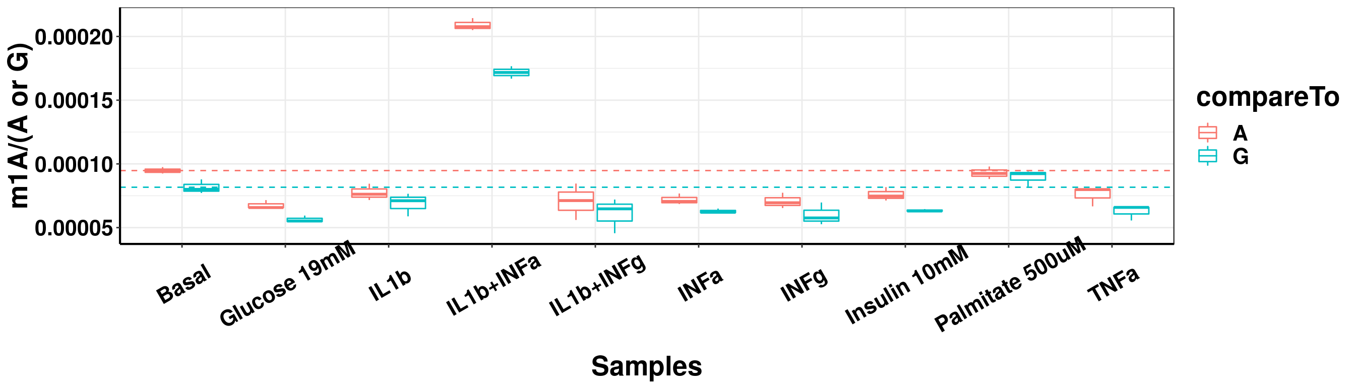
### Individual HP-19038-01 and SAMN10977276
library(ggplot2)
library(ggpubr)

### quantify A
A_quant <- read.table("~/Rohit_T1D/Human_Islet_Stimu_QQQ/T1D_20190517_A.txt", sep = "\t", header = T, stringsAsFactors = F)[-c(1),c("Sample.Name","Sample.Type","Actual.Concentration","Area")]

for( i in 1:(nrow(A_quant)-1) ){ A_quant$group[i] <- (A_quant$Sample.Type[i]!=A_quant$Sample.Type[i+1] ) }

num_SampleGroup <- sum( A_quant$group)-1

Samples <- data.frame(start= (which(A_quant$group )+1)[1:num_SampleGroup], end = which(A_quant$group)[-c(1)])[seq(1,num_SampleGroup,2),]

result_A <- result_m6A <- result_G <- result_m1A <- NULL
for(i in 1:nrow(Samples) ){
  std_ID <- c( (Samples$start[i]-5):( Samples$start[i]-1), (Samples$end[i]+1):( Samples$end[i]+5))
  A_quant_std <- dplyr::mutate_if(A_quant[std_ID,c("Actual.Concentration","Area")], is.character , as.numeric )
  A_quant_tmp <-data.frame(Area = A_quant[Samples$start[i]:Samples$end[i],c("Area")])
  fit <- lm(Actual.Concentration~Area, A_quant_std)
  result_A <- rbind(result_A,cbind( "Name"= A_quant$Sample.Name[Samples$start[i]:Samples$end[i]], "A"=  predict(fit, newdata = A_quant_tmp) ) )
}

### quantify G
G_quant <- read.table("~/Rohit_T1D/Human_Islet_Stimu_QQQ/T1D_20190517_G.txt", sep = "\t", header = T, stringsAsFactors = F)[-c(1),c("Sample.Name","Sample.Type","Actual.Concentration","Area")]

for(i in 1:nrow(Samples) ){
  std_ID <- c( (Samples$start[i]-5):( Samples$start[i]-1), (Samples$end[i]+1):( Samples$end[i]+5))
  G_quant_std <- dplyr::mutate_if(G_quant[std_ID,c("Actual.Concentration","Area")], is.character , as.numeric )
  G_quant_tmp <-data.frame(Area = G_quant[Samples$start[i]:Samples$end[i],c("Area")])
  fit <- lm(Actual.Concentration~Area, G_quant_std)
  result_G <- rbind(result_G,cbind( "Name"= G_quant$Sample.Name[Samples$start[i]:Samples$end[i]], "G"=  predict(fit, newdata = G_quant_tmp) ) )
}

### quantify m6A
m6A_quant <- read.table("~/Rohit_T1D/Human_Islet_Stimu_QQQ/T1D_20190517_m6A.txt", sep = "\t", header = T, stringsAsFactors = F)[-c(1),c("Sample.Name","Sample.Type","Actual.Concentration","Area")]

for(i in 1:nrow(Samples) ){
  std_ID <- c( (Samples$start[i]-5):( Samples$start[i]-1), (Samples$end[i]+1):( Samples$end[i]+5))
  m6A_quant_std <- dplyr::mutate_if(m6A_quant[std_ID,c("Actual.Concentration","Area")], is.character , as.numeric )
  m6A_quant_tmp <-data.frame(Area = m6A_quant[Samples$start[i]:Samples$end[i],c("Area")])
  fit <- lm(Actual.Concentration~Area, m6A_quant_std)
  result_m6A <- rbind(result_m6A,cbind( "Name"= m6A_quant$Sample.Name[Samples$start[i]:Samples$end[i]], "m6A"=  predict(fit, newdata = m6A_quant_tmp) ) )
}

### quantify m1A
m1A_quant <- read.table("~/Rohit_T1D/Human_Islet_Stimu_QQQ/T1D_20190517_m1A.txt", sep = "\t", header = T, stringsAsFactors = F)[-c(1),c("Sample.Name","Sample.Type","Actual.Concentration","Area")]

for(i in 1:nrow(Samples) ){
  std_ID <- c( (Samples$start[i]-5):( Samples$start[i]-1), (Samples$end[i]+1):( Samples$end[i]+5))
  m1A_quant_std <- dplyr::mutate_if(m1A_quant[std_ID,c("Actual.Concentration","Area")], is.character , as.numeric )
  m1A_quant_tmp <-data.frame(Area = m1A_quant[Samples$start[i]:Samples$end[i],c("Area")])
  fit <- lm(Actual.Concentration~Area, m1A_quant_std)
  result_m1A <- rbind(result_m1A,cbind( "Name"= m1A_quant$Sample.Name[Samples$start[i]:Samples$end[i]], "m1A"=  predict(fit, newdata = m1A_quant_tmp) ) )
}


result_batch3 <- data.frame( sampleName = rep( c("Basal", "Glucose 19mM","Insulin 10mM", "Palmitate 500uM","IL1b","INFa","INFg","TNFa","IL1b+INFa","IL1b+INFg"), 3) , A = as.numeric(result_A[1:30,2]), G = as.numeric(result_G[1:30,2]), m6A = as.numeric(result_m6A[1:30,2]), m1A =  as.numeric(result_m1A[1:30,2]) )
result_batch3$m6AvsA <- result_batch3$m6A/result_batch3$A
result_batch3$m6AvsG <- result_batch3$m6A/result_batch3$G
result_batch3$m1AvsA <- result_batch3$m1A/result_batch3$A
result_batch3$m1AvsG <- result_batch3$m1A/result_batch3$G

result_batch4 <- data.frame( sampleName = rep( c("Basal", "Glucose 19mM","Insulin 10mM", "Palmitate 500uM","IL1b","INFa","INFg","TNFa","IL1b+INFa","IL1b+INFg"), 3) , A = as.numeric(result_A[31:60,2]), G = as.numeric(result_G[31:60,2]), m6A = as.numeric(result_m6A[31:60,2]), m1A =  as.numeric(result_m1A[31:60,2]) )
result_batch4$m6AvsA <- result_batch4$m6A/result_batch4$A
result_batch4$m6AvsG <- result_batch4$m6A/result_batch4$G
result_batch4$m1AvsA <- result_batch4$m1A/result_batch4$A
result_batch4$m1AvsG <- result_batch4$m1A/result_batch4$G
HP-19038-01
DT::datatable(result_batch3, options = list(scrollX = TRUE, keys = TRUE, pageLength = 10),rownames = F)result_batch3_m6A_melt <- data.frame(sampleName = rep(result_batch3$sampleName,2), m6A = c(result_batch3$m6AvsA,result_batch3$m6AvsG), compareTo = c(rep("A",nrow(result_batch3) ),rep("G",nrow(result_batch3))) )
ggplot(result_batch3_m6A_melt,aes( x = sampleName, y = m6A, color = compareTo))+geom_boxplot( )+ xlab("Samples") +ylab("m6A/(A or G)")+theme_bw()+theme(text = element_text(face = "bold", size = 20, color = "black"),axis.text = element_text(face = "bold", size = 16, color = "black"),axis.text.x = element_text(angle = 30,vjust = 0.7), axis.line = element_line(colour = "black", size = 0.75))+geom_abline(intercept = mean(result_batch3$m6AvsA[result_batch3$sampleName=="Basal"]), slope = 0, lty = "dashed", colour ="#F8766D" )+geom_abline(intercept = mean(result_batch3$m6AvsG[result_batch3$sampleName=="Basal"]), slope = 0, lty = "dashed", colour ="#00BFC4" )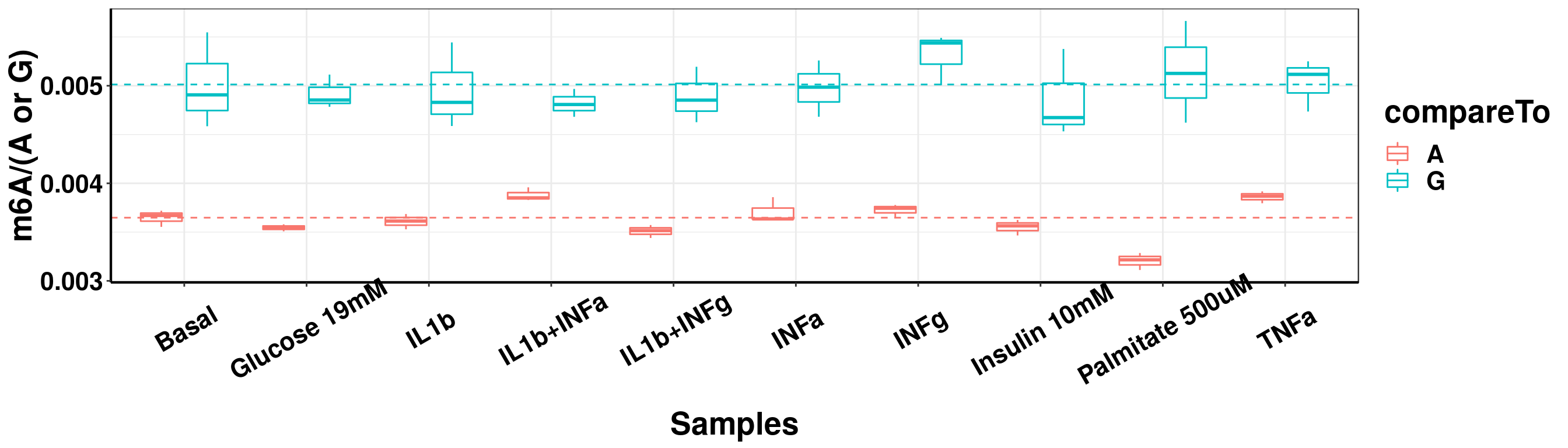
| Version | Author | Date |
|---|---|---|
| 2616200 | scottzijiezhang | 2019-05-20 |
result_batch3_m1A_melt <- data.frame(sampleName = rep(result_batch3$sampleName,2), m1A = c(result_batch3$m1AvsA,result_batch3$m1AvsG), compareTo = c(rep("A",nrow(result_batch3) ),rep("G",nrow(result_batch3))) )
ggplot(result_batch3_m1A_melt,aes( x = sampleName, y = m1A, colour = compareTo))+geom_boxplot( )+ xlab("Samples") +ylab("m1A/(A or G)")+theme_bw()+theme(text = element_text(face = "bold", size = 20, color = "black"),axis.text = element_text(face = "bold", size = 16, color = "black"),axis.text.x = element_text(angle = 30,vjust = 0.7), axis.line = element_line(colour = "black", size = 0.75))+geom_abline(intercept = mean(result_batch3$m1AvsA[result_batch3$sampleName=="Basal"]), slope = 0, lty = "dashed", colour ="#F8766D"  )+geom_abline(intercept = mean(result_batch3$m1AvsG[result_batch3$sampleName=="Basal"]), slope = 0, lty = "dashed", colour ="#00BFC4"  )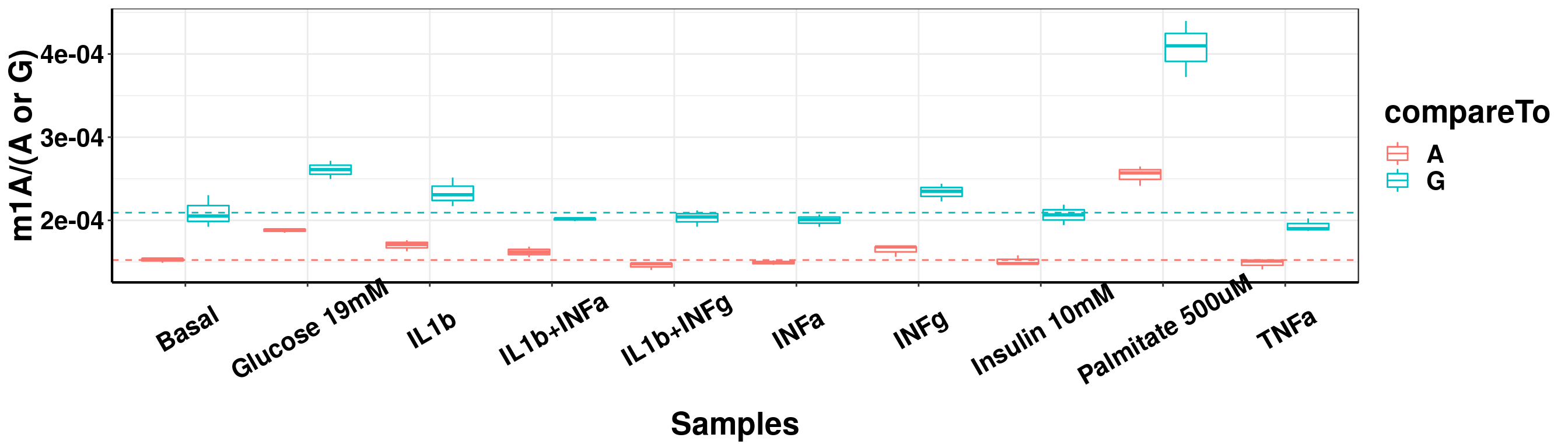
| Version | Author | Date |
|---|---|---|
| 2616200 | scottzijiezhang | 2019-05-20 |
SAMN10977276
DT::datatable(result_batch4, options = list(scrollX = TRUE, keys = TRUE, pageLength = 10),rownames = F)result_batch4_m6A_melt <- data.frame(sampleName = rep(result_batch4$sampleName,2), m6A = c(result_batch4$m6AvsA,result_batch4$m6AvsG), compareTo = c(rep("A",nrow(result_batch4) ),rep("G",nrow(result_batch4))) )
ggplot(result_batch4_m6A_melt,aes( x = sampleName, y = m6A, color = compareTo))+geom_boxplot( )+ xlab("Samples") +ylab("m6A/(A or G)")+theme_bw()+theme(text = element_text(face = "bold", size = 20, color = "black"),axis.text = element_text(face = "bold", size = 16, color = "black"),axis.text.x = element_text(angle = 30,vjust = 0.7), axis.line = element_line(colour = "black", size = 0.75))+geom_abline(intercept = mean(result_batch4$m6AvsA[result_batch4$sampleName=="Basal"]), slope = 0, lty = "dashed", colour ="#F8766D" )+geom_abline(intercept = mean(result_batch4$m6AvsG[result_batch4$sampleName=="Basal"]), slope = 0, lty = "dashed", colour ="#00BFC4" )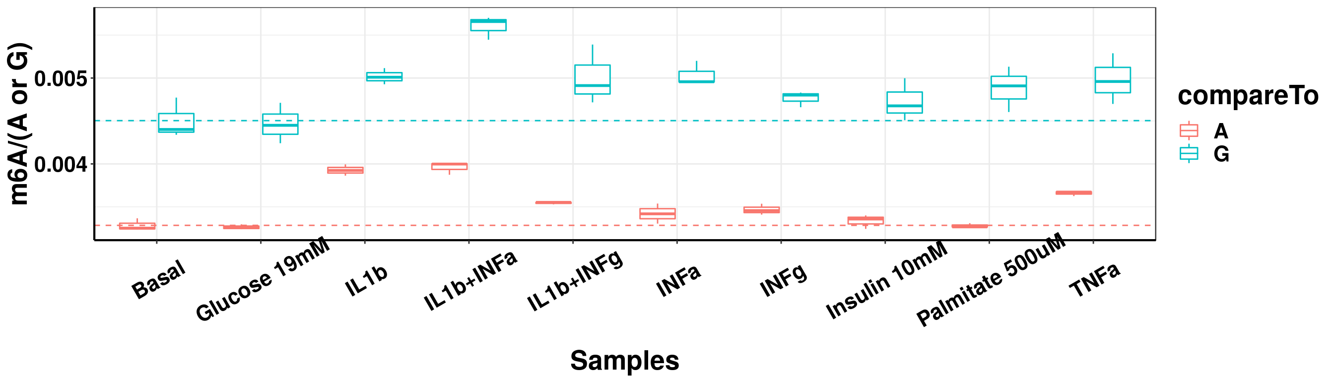
| Version | Author | Date |
|---|---|---|
| 2616200 | scottzijiezhang | 2019-05-20 |
result_batch4_m1A_melt <- data.frame(sampleName = rep(result_batch4$sampleName,2), m1A = c(result_batch4$m1AvsA,result_batch4$m1AvsG), compareTo = c(rep("A",nrow(result_batch4) ),rep("G",nrow(result_batch4))) )
ggplot(result_batch4_m1A_melt,aes( x = sampleName, y = m1A, colour = compareTo))+geom_boxplot( )+ xlab("Samples") +ylab("m1A/(A or G)")+theme_bw()+theme(text = element_text(face = "bold", size = 20, color = "black"),axis.text = element_text(face = "bold", size = 16, color = "black"),axis.text.x = element_text(angle = 30,vjust = 0.7), axis.line = element_line(colour = "black", size = 0.75))+geom_abline(intercept = mean(result_batch4$m1AvsA[result_batch4$sampleName=="Basal"]), slope = 0, lty = "dashed", colour ="#F8766D"  )+geom_abline(intercept = mean(result_batch4$m1AvsG[result_batch4$sampleName=="Basal"]), slope = 0, lty = "dashed", colour ="#00BFC4"  )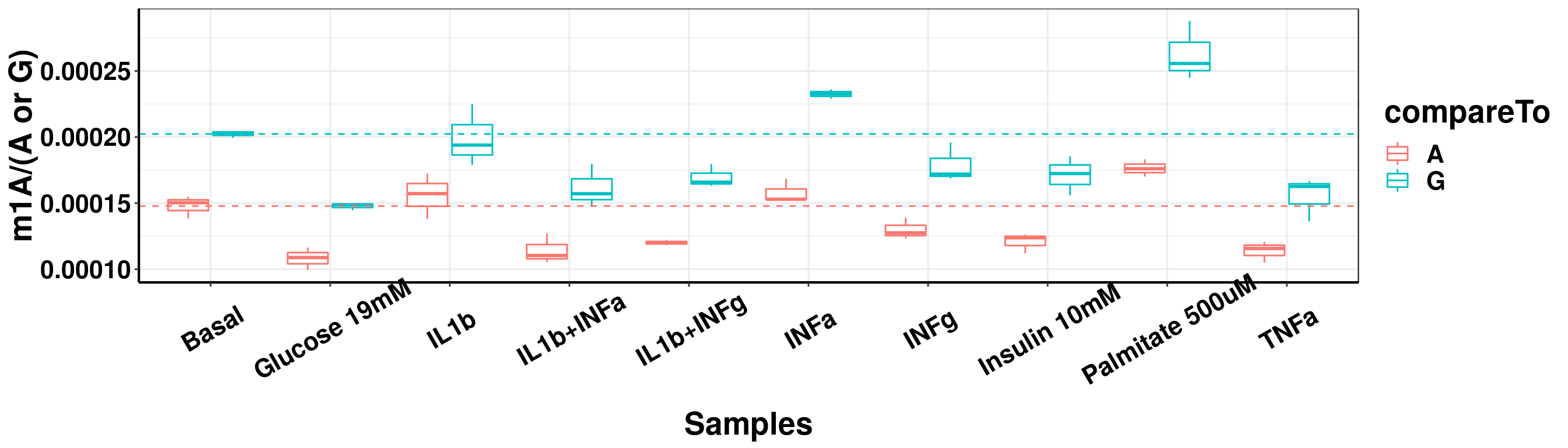
| Version | Author | Date |
|---|---|---|
| 2616200 | scottzijiezhang | 2019-05-20 |
Normalize batch1 and batch2 data to last batch of data and show all.
Since different batch of samples were run using different standard set, I normalized the basal conditon so that they are comparable. The first batch had very large standard error because the QQQ machine wasn’t very stable. The later three batches were ran after the machine was tuned and is much more reliable.
basalMean_m6A <- mean(c(result_batch3[result_batch3$sampleName =="Basal","m6AvsA"], result_batch4[result_batch3$sampleName =="Basal","m6AvsA"]))
sizeFactor_m6A <- c(mean(result_batch1[result_batch1$sampleName =="Basal","m6AvsA"]),
                    mean(result_batch2[result_batch1$sampleName =="Basal","m6AvsA"]),
                    mean(result_batch3[result_batch1$sampleName =="Basal","m6AvsA"]),
                    mean(result_batch4[result_batch1$sampleName =="Basal","m6AvsA"]))/basalMean_m6A

all_m6A <- data.frame( condition = rep( levels(result_batch1$sampleName), 4),
                       sample = c(rep("HP-19026-01",10),rep("HP-19030-01",10),rep("HP-19038-01",10),rep("SAMN10977276",10)),
                       m6AvsA = c( tapply(result_batch1$m6AvsA,result_batch1$sampleName,mean)/sizeFactor_m6A[1],
                                   tapply(result_batch2$m6AvsA,result_batch2$sampleName,mean)/sizeFactor_m6A[2],
                                   tapply(result_batch3$m6AvsA,result_batch3$sampleName,mean)/sizeFactor_m6A[3],
                                   tapply(result_batch4$m6AvsA,result_batch4$sampleName,mean)/sizeFactor_m6A[4]),
                       sd = c( tapply(result_batch1$m6AvsA,result_batch1$sampleName,sd)/sizeFactor_m6A[1],
                                   tapply(result_batch2$m6AvsA,result_batch2$sampleName,sd)/sizeFactor_m6A[2],
                                   tapply(result_batch3$m6AvsA,result_batch3$sampleName,sd)/sizeFactor_m6A[3],
                                   tapply(result_batch4$m6AvsA,result_batch4$sampleName,sd)/sizeFactor_m6A[4])
                       )


ggplot(all_m6A, aes(x = condition, y = m6AvsA*100, fill = sample))+geom_bar(stat = "identity", position=position_dodge() )+ylab("m6A/A Ratio (%)")+
  geom_errorbar(aes(ymin = (m6AvsA-sd)*100, ymax = (m6AvsA+sd)*100 ) , width = 0.5, position=position_dodge(0.9)  )+ theme_bw()  + xlab("Features")+
    geom_hline(yintercept = 0,linetype="dotted", colour = "red")+theme(axis.ticks = element_blank(), panel.border = element_blank(),
                     panel.grid.minor = element_blank(), axis.line = element_line(colour = "black"), axis.text.x = element_text(face="bold",size = 18, colour = "black",hjust = 0.3, angle = -20),axis.text.y = element_text(face="bold",size =25),axis.title.x = element_blank(), axis.title.y = element_text(face="bold",size =25) )+geom_abline(intercept = mean(all_m6A$m6AvsA[all_m6A$condition == "Basal"])*100, slope = 0, lty = "dashed", colour ="#00BFC4"  )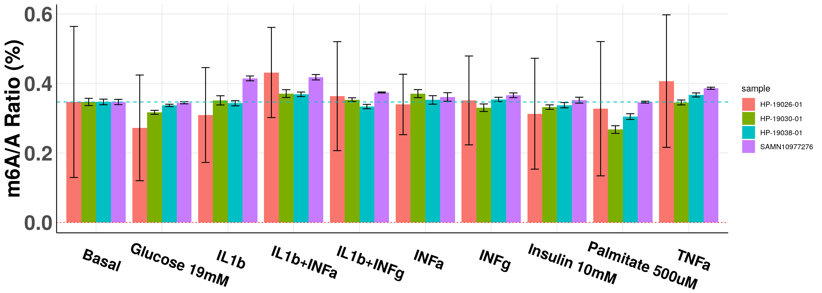
basalMean_m1A <- mean(c(result_batch3[result_batch3$sampleName =="Basal","m1AvsA"], result_batch4[result_batch3$sampleName =="Basal","m1AvsA"]) )
sizeFactor_m1A <- c(mean(result_batch2[result_batch1$sampleName =="Basal","m1AvsA"]),
                    mean(result_batch3[result_batch1$sampleName =="Basal","m1AvsA"]),
                    mean(result_batch4[result_batch1$sampleName =="Basal","m1AvsA"]))/basalMean_m1A

all_m1A <- data.frame( condition = rep( levels(result_batch1$sampleName), 3),
                       sample = c(rep("HP-19030-01",10),rep("HP-19038-01",10),rep("SAMN10977276",10)),
                       m1AvsA = c( tapply(result_batch2$m1AvsA,result_batch1$sampleName,mean)/sizeFactor_m1A[1],
                                   tapply(result_batch3$m1AvsA,result_batch2$sampleName,mean)/sizeFactor_m1A[2],
                                   tapply(result_batch4$m1AvsA,result_batch3$sampleName,mean)/sizeFactor_m1A[3]),
                       sd = c(     tapply(result_batch2$m1AvsA,result_batch2$sampleName,sd)/sizeFactor_m6A[1],
                                   tapply(result_batch3$m1AvsA,result_batch3$sampleName,sd)/sizeFactor_m6A[2],
                                   tapply(result_batch4$m1AvsA,result_batch4$sampleName,sd)/sizeFactor_m6A[3])
                       )


ggplot(all_m1A, aes(x = condition, y = m1AvsA*100, fill = sample))+geom_bar(stat = "identity", position=position_dodge() )+ylab("m1A/A Ratio (%)")+
  geom_errorbar(aes(ymin =( m1AvsA-sd)*100, ymax = (m1AvsA+sd)*100 ) , width = 0.5, position=position_dodge(0.9)  )+ theme_bw()  + xlab("Features")+
    geom_hline(yintercept = 0,linetype="dotted", colour = "red")+theme(axis.ticks = element_blank(), panel.border = element_blank(),
                     panel.grid.minor = element_blank(), axis.line = element_line(colour = "black"), axis.text.x = element_text(face="bold",size = 18, colour = "black",hjust = 0.3, angle = -20),axis.text.y = element_text(face="bold",size =25),axis.title.x = element_blank(), axis.title.y = element_text(face="bold",size =25) )+geom_abline(intercept = mean(all_m1A$m1AvsA[all_m1A$condition == "Basal"])*100, slope = 0, lty = "dashed", colour ="#00BFC4"  )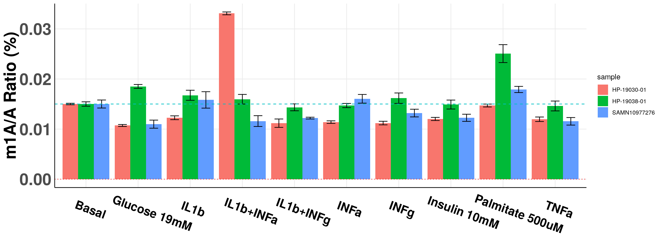
The earlier batch of HP=19026-1 has very large technical variation because the QQQ machine wasn’t in a good condition at that time. So I re-masured this batch later after we tuned the QQQ machine. The new batch has much smaller technical variation. ### Individual HP-19026-01
library(ggplot2)
library(ggpubr)

### quantify A
A_quant <- read.table("~/Rohit_T1D/Human_Islet_Stimu_QQQ/20190521_T1D_A.txt", sep = "\t", header = T, stringsAsFactors = F)[1:50,c("Sample.Name","Sample.Type","Actual.Concentration","Area")]

for( i in 1:(nrow(A_quant)-1) ){ A_quant$group[i] <- (A_quant$Sample.Type[i]!=A_quant$Sample.Type[i+1] ) }

num_SampleGroup <- sum( A_quant$group)-1

Samples <- data.frame(start= (which(A_quant$group )+1)[1:num_SampleGroup], end = which(A_quant$group)[-c(1)])[seq(1,num_SampleGroup,2),]

result_A <- result_m6A <- result_m1A <- NULL
for(i in 1:nrow(Samples) ){
  std_ID <- c( (Samples$start[i]-5):( Samples$start[i]-1), (Samples$end[i]+1):( Samples$end[i]+5))
  A_quant_std <- dplyr::mutate_if(A_quant[std_ID,c("Actual.Concentration","Area")], is.character , as.numeric )
  A_quant_tmp <-data.frame(Area = A_quant[Samples$start[i]:Samples$end[i],c("Area")])
  fit <- lm(Actual.Concentration~Area, A_quant_std)
  result_A <- rbind(result_A,cbind( "Name"= A_quant$Sample.Name[Samples$start[i]:Samples$end[i]], "A"=  predict(fit, newdata = A_quant_tmp) ) )
}

### quantify m6A
m6A_quant <- read.table("~/Rohit_T1D/Human_Islet_Stimu_QQQ/20190521_T1D_m6A.txt", sep = "\t", header = T, stringsAsFactors = F)[1:50,c("Sample.Name","Sample.Type","Actual.Concentration","Area")]

for(i in 1:nrow(Samples) ){
  std_ID <- c( (Samples$start[i]-5):( Samples$start[i]-1), (Samples$end[i]+1):( Samples$end[i]+5))
  m6A_quant_std <- dplyr::mutate_if(m6A_quant[std_ID,c("Actual.Concentration","Area")], is.character , as.numeric )
  m6A_quant_tmp <-data.frame(Area = m6A_quant[Samples$start[i]:Samples$end[i],c("Area")])
  fit <- lm(Actual.Concentration~Area, m6A_quant_std)
  result_m6A <- rbind(result_m6A,cbind( "Name"= m6A_quant$Sample.Name[Samples$start[i]:Samples$end[i]], "m6A"=  predict(fit, newdata = m6A_quant_tmp) ) )
}

### quantify m1A
m1A_quant <- read.table("~/Rohit_T1D/Human_Islet_Stimu_QQQ/20190521_T1D_m1A.txt", sep = "\t", header = T, stringsAsFactors = F)[1:50,c("Sample.Name","Sample.Type","Actual.Concentration","Area")]

for(i in 1:nrow(Samples) ){
  std_ID <- c( (Samples$start[i]-5):( Samples$start[i]-1), (Samples$end[i]+1):( Samples$end[i]+5))
  m1A_quant_std <- dplyr::mutate_if(m1A_quant[std_ID,c("Actual.Concentration","Area")], is.character , as.numeric )
  m1A_quant_tmp <-data.frame(Area = m1A_quant[Samples$start[i]:Samples$end[i],c("Area")])
  fit <- lm(Actual.Concentration~Area, m1A_quant_std)
  result_m1A <- rbind(result_m1A,cbind( "Name"= m1A_quant$Sample.Name[Samples$start[i]:Samples$end[i]], "m1A"=  predict(fit, newdata = m1A_quant_tmp) ) )
}


result_batch1 <- data.frame( sampleName = rep( c("Basal", "Glucose 19mM","Insulin 10mM", "Palmitate 500uM","IL1b","INFa","INFg","TNFa","IL1b+INFa","IL1b+INFg"), 3) , A = as.numeric(result_A[1:30,2]), m1A = as.numeric(result_m1A[1:30,2]), m6A = as.numeric(result_m6A[1:30,2]) )
result_batch1$m6AvsA <- result_batch1$m6A/result_batch1$A
result_batch1$m1AvsA <- result_batch1$m1A/result_batch1$A


DT::datatable(result_batch1, options = list(scrollX = TRUE, keys = TRUE, pageLength = 10),rownames = F)
ggplot(result_batch1,aes( x = sampleName, y = m6AvsA))+geom_boxplot( )+ xlab("Samples") +ylab("m6A/A")+theme_bw()+theme(text = element_text(face = "bold", size = 20, color = "black"),axis.text = element_text(face = "bold", size = 16, color = "black"),axis.text.x = element_text(angle = 30,vjust = 0.7), axis.line = element_line(colour = "black", size = 0.75))Warning: Removed 1 rows containing non-finite values (stat_boxplot).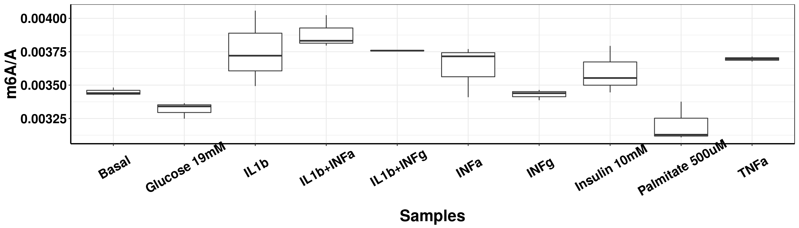
| Version | Author | Date |
|---|---|---|
| ce13e24 | scottzijiezhang | 2020-08-13 |
New sumarized data with updated HP-19026-01 measurement.
library(ggsci)

## calculate a size factor to correct the variation of overal measurement in batch2 sample due to standard set used in that batch.
basalMean_m6A <- mean(c(result_batch1[result_batch3$sampleName =="Basal","m6AvsA"],result_batch3[result_batch3$sampleName =="Basal","m6AvsA"], result_batch4[result_batch3$sampleName =="Basal","m6AvsA"]))
sizeFactor_m6A <-  mean(result_batch2[result_batch1$sampleName =="Basal","m6AvsA"])/basalMean_m6A

all_m6A_new <- data.frame( condition = rep( levels(result_batch1$sampleName), 4),
                       sample = c(rep("HP-19026-01",10),rep("HP-19030-01",10),rep("HP-19038-01",10),rep("SAMN10977276",10)),
                       m6AvsA = c( tapply(result_batch1$m6AvsA,result_batch1$sampleName,mean, na.rm = T),
                                   tapply(result_batch2$m6AvsA,result_batch2$sampleName,mean)/sizeFactor_m6A,
                                   tapply(result_batch3$m6AvsA,result_batch3$sampleName,mean),
                                   tapply(result_batch4$m6AvsA,result_batch4$sampleName,mean) ),
                       sd = c( tapply(result_batch1$m6AvsA,result_batch1$sampleName,sd, na.rm = T),
                                   tapply(result_batch2$m6AvsA,result_batch2$sampleName,sd)/sizeFactor_m6A,
                                   tapply(result_batch3$m6AvsA,result_batch3$sampleName,sd),
                                   tapply(result_batch4$m6AvsA,result_batch4$sampleName,sd))
                       )

ggplot(all_m6A_new, aes(x = condition, y = m6AvsA*100, fill = sample))+geom_bar(stat = "identity", position=position_dodge() )+ylab("m6A/A Ratio (%)")+
  geom_errorbar(aes(ymin = (m6AvsA-sd)*100, ymax = (m6AvsA+sd)*100 ) , width = 0.5, position=position_dodge(0.9)  )+ theme_bw()  + xlab("Features")+
    geom_hline(yintercept = 0,linetype="dotted", colour = "red")+theme(axis.ticks = element_blank(), panel.border = element_blank(),
                     panel.grid.minor = element_blank(), axis.line = element_line(colour = "black"), axis.text.x = element_text(face="bold",size = 18, colour = "black",hjust = 0.3, angle = -20),axis.text.y = element_text(face="bold",size =25, color = "black"),axis.title.x = element_blank(), axis.title.y = element_text(face="bold",size =25) )+geom_abline(intercept = mean(all_m6A$m6AvsA[all_m6A$condition == "Basal"])*100, slope = 0, lty = "dashed", colour ="#00BFC4"  )+scale_fill_jco()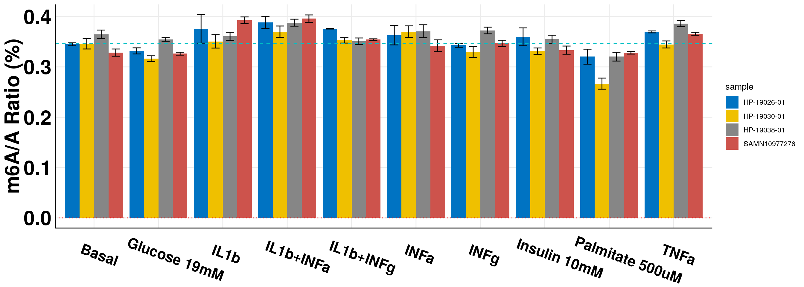
| Version | Author | Date |
|---|---|---|
| ce13e24 | scottzijiezhang | 2020-08-13 |
cbbPalette <- c( "#E69F00", "#56B4E9", "#009E73", "#F0E442", "#0072B2", "#D55E00", "#CC79A7")

m6A_toBasal <- dplyr::filter(all_m6A_new, condition %in% c("IL1b","INFa","INFg","TNFa","IL1b+INFa","IL1b+INFg") )
m6A_toBasal$m6AvsA <- m6A_toBasal$m6AvsA/rep( dplyr::filter(all_m6A_new, condition =="Basal" )$m6AvsA, c(6,6,6,6) )

m6A_toBasal$condition <- factor(m6A_toBasal$condition, levels = c("IL1b","INFa","INFg","TNFa","IL1b+INFa","IL1b+INFg") )

ggplot( m6A_toBasal, aes( x= condition, y = m6AvsA*100 , fill = condition) )+geom_boxplot(size = 0.9)+ylab("m6A/A Ratio \n(% to Basal condition)")+
   theme_bw()  + xlab("Condition")+theme(axis.ticks = element_line(color = "black"), panel.border = element_blank(),
                     panel.grid.minor = element_blank(), axis.line = element_line(colour = "black"), axis.text.x = element_text( size = 14, colour = "black",hjust = 0.9, angle = 30 ),axis.text.y = element_text( size =14, color = "black"),axis.title.x = element_blank(), axis.title.y = element_text( size =14), legend.position = "none" , panel.grid = element_blank())+geom_abline(intercept = mean(all_m6A$m6AvsA[all_m6A$condition == "Basal"])*100, slope = 0, lty = "dashed", colour ="#00BFC4"  )+scale_fill_manual(values = cbbPalette)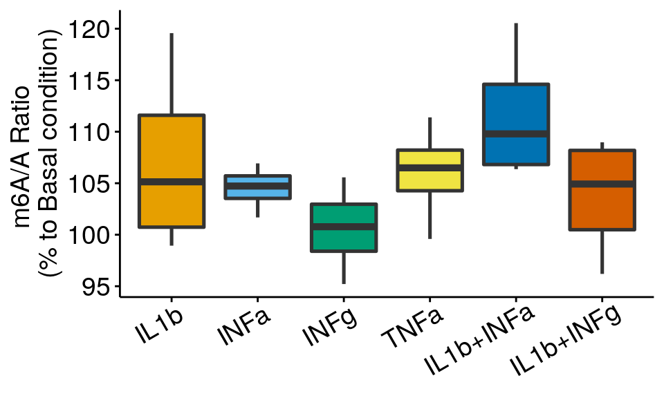
| Version | Author | Date |
|---|---|---|
| ce13e24 | scottzijiezhang | 2020-08-13 |
m6A_toBasal_collapse <- data.frame( condition = names( tapply(m6A_toBasal$m6AvsA, m6A_toBasal$condition, function(x) sqrt(var(x)/length(x)) ) ),
                                    ratio = tapply(m6A_toBasal$m6AvsA, m6A_toBasal$condition, mean ),
                                    sem = tapply(m6A_toBasal$m6AvsA, m6A_toBasal$condition, function(x) sqrt(var(x)/length(x)) )
                                    )
ggplot( m6A_toBasal_collapse, aes( x= condition, y = ratio*100 , fill = condition) )+geom_bar(stat = "identity", color = "black")+ylab("m6A/A Ratio \n(% to Basal condition)")+geom_errorbar(aes(ymin = (ratio-sem)*100, ymax = (ratio+sem)*100 ) , width = 0.5, position=position_dodge(0.9)  )+geom_abline(intercept = 100, slope = 0, lty = "dashed", colour ="black"  )+
   theme_bw()  + xlab("Condition")+theme(axis.ticks = element_line(color = "black"), panel.border = element_blank(),
                     panel.grid.minor = element_blank(), axis.line = element_line(colour = "black"), axis.text.x = element_text( size = 14, colour = "black",hjust = 0.9, angle = 30 ),axis.text.y = element_text( size =14, color = "black"),axis.title.x = element_blank(), axis.title.y = element_text( size =14), legend.position = "none" , panel.grid = element_blank()) +scale_fill_manual(values = cbbPalette)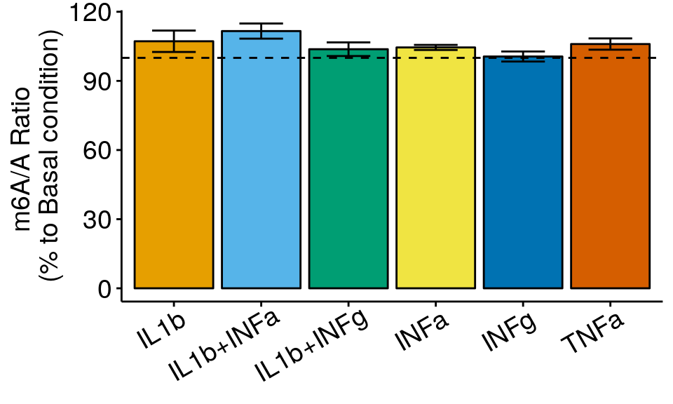
| Version | Author | Date |
|---|---|---|
| ba4b639 | scottzijiezhang | 2020-08-15 |
I have use two types of plots above. In the boxplot, the lower and upper hinges correspond to the first and third quartiles. The horizontal line indicates the median and the whiskers correspond to the value no further than 1.5× the interquartile range. In the barplot, the error bars are standard error of mean computed from distribution of means (from technical replicates).
m6A_toBasal_glu <- dplyr::filter(all_m6A_new, condition %in% c("Glucose 19mM", "Palmitate 500uM") )
m6A_toBasal_glu$m6AvsA <- m6A_toBasal_glu$m6AvsA/rep( dplyr::filter(all_m6A_new, condition =="Basal" )$m6AvsA, c(2,2,2,2) )

m6A_toBasal_glu$condition <- factor(m6A_toBasal_glu$condition, levels = c("Glucose 19mM", "Palmitate 500uM") )

ggplot( m6A_toBasal_glu, aes( x= condition, y = m6AvsA*100 , fill = condition) )+geom_boxplot(size = 0.9)+ylab("m6A/A Ratio \n(% to Basal condition)")+
   theme_bw()  + xlab("Condition")+theme(axis.ticks = element_line(color = "black"), panel.border = element_blank(),
                     panel.grid.minor = element_blank(), axis.line = element_line(colour = "black"), axis.text.x = element_text( size = 14, colour = "black",hjust = 0.9, angle = 30 ),axis.text.y = element_text( size =14, color = "black"),axis.title.x = element_blank(), axis.title.y = element_text( size =14), legend.position = "none" , panel.grid = element_blank())+geom_abline(intercept = mean(all_m6A$m6AvsA[all_m6A$condition == "Basal"])*100, slope = 0, lty = "dashed", colour ="#00BFC4"  )+scale_fill_manual(values = cbbPalette)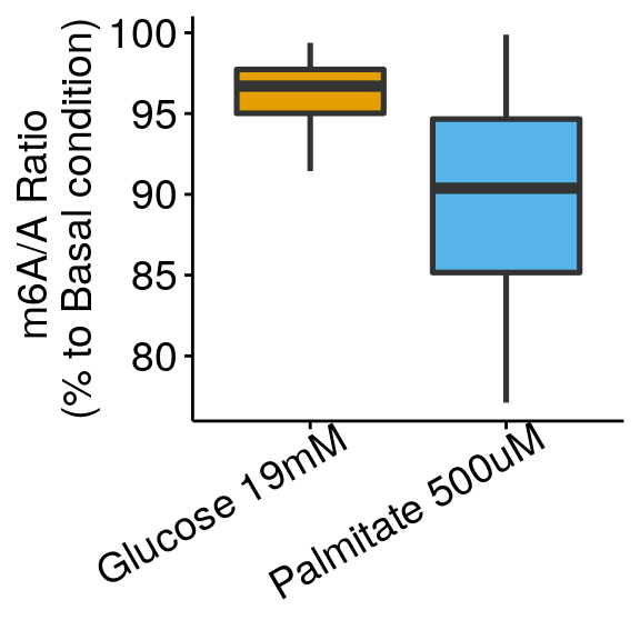
m6A_toBasal_glu_collapse <- data.frame( condition = names( tapply(m6A_toBasal_glu$m6AvsA, m6A_toBasal_glu$condition, function(x) sqrt(var(x)/length(x)) ) ),
                                    ratio = tapply(m6A_toBasal_glu$m6AvsA, m6A_toBasal_glu$condition, mean ),
                                    sem = tapply(m6A_toBasal_glu$m6AvsA, m6A_toBasal_glu$condition, function(x) sqrt(var(x)/length(x)) )
                                    )
ggplot( m6A_toBasal_glu_collapse, aes( x= condition, y = ratio*100 , fill = condition) )+geom_bar(stat = "identity", color = "black")+ylab("m6A/A Ratio \n(% to Basal condition)")+geom_errorbar(aes(ymin = (ratio-sem)*100, ymax = (ratio+sem)*100 ) , width = 0.5, position=position_dodge(0.9)  )+geom_abline(intercept = 100, slope = 0, lty = "dashed", colour ="black"  )+
   theme_bw()  + xlab("Condition")+theme(axis.ticks = element_line(color = "black"), panel.border = element_blank(),
                     panel.grid.minor = element_blank(), axis.line = element_line(colour = "black"), axis.text.x = element_text( size = 14, colour = "black",hjust = 0.9, angle = 30 ),axis.text.y = element_text( size =14, color = "black"),axis.title.x = element_blank(), axis.title.y = element_text( size =14), legend.position = "none" , panel.grid = element_blank()) +scale_fill_manual(values = cbbPalette)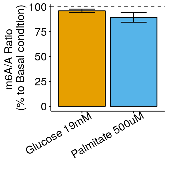
Paired comparasion
I used paired t-test for statistics of paired comparison.
library(ggpubr)
cbbPalette <- c( "#E69F00", "#56B4E9", "#009E73", "#F0E442", "#0072B2", "#D55E00", "#CC79A7")

basalILIN <- dplyr::filter(all_m6A_new, condition %in% c("Basal","IL1b+INFa") )
basalILIN <- basalILIN[order(  basalILIN$condition), ]

ggplot(data =  basalILIN, mapping = aes( x= condition, y = m6AvsA*100 , color = sample, shape = condition, group = sample ) )+geom_line( size = 1)+geom_point( size = 3 )+
  ylab("m6A/A Ratio (%)")+
   theme_bw()  + xlab("Condition")+theme(axis.ticks = element_line(color = "black"), panel.border = element_blank(),
                     panel.grid.minor = element_blank(), axis.line = element_line(colour = "black"), axis.text.x = element_text( size = 15, colour = "black",hjust = 0.9, angle = 30 ),axis.text.y = element_text( size =15, color = "black"),axis.title.x = element_blank(), axis.title.y = element_text( size =15),  panel.grid = element_blank(), legend.text = element_text(size = 15), legend.title = element_text(size = 15) )+scale_color_manual(values = cbbPalette[-c(4)] )+scale_shape_discrete(guide = FALSE)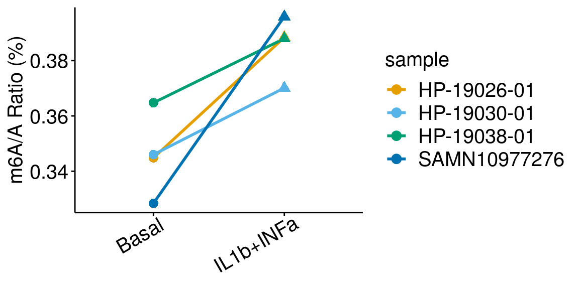
DT::datatable( compare_means(m6AvsA ~ condition, data = basalILIN,
               paired = TRUE , method = "t.test"), rownames = FALSE )
basalILINg <- dplyr::filter(all_m6A_new, condition %in% c("Basal","IL1b+INFg") )
ggplot(data = basalILINg, mapping = aes( x= condition, y = m6AvsA*100 , color = sample, shape = condition, group = sample ) )+geom_line( size = 1)+geom_point( size = 3 )+
ylab("m6A/A Ratio (%)")+
theme_bw() + xlab("Condition")+theme(axis.ticks = element_line(color = "black"), panel.border = element_blank(),
panel.grid.minor = element_blank(), axis.line = element_line(colour = "black"), axis.text.x = element_text( size = 15, colour = "black",hjust = 0.9, angle = 30 ),axis.text.y = element_text( size =15, color = "black"),axis.title.x = element_blank(), axis.title.y = element_text( size =15), panel.grid = element_blank(), legend.text = element_text(size = 15), legend.title = element_text(size = 15) )+scale_color_manual(values = cbbPalette[-c(4)] )+scale_shape_discrete(guide = FALSE)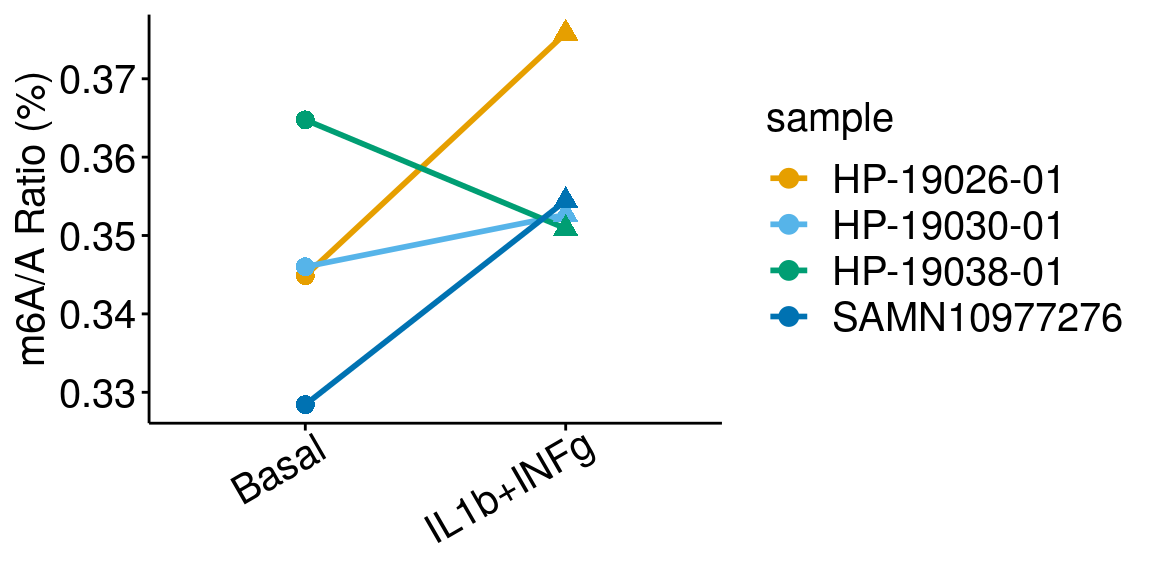
| Version | Author | Date |
|---|---|---|
| ce13e24 | scottzijiezhang | 2020-08-13 |
DT::datatable( compare_means(m6AvsA ~ condition, data = basalILINg,
               paired = TRUE , method = "t.test"), rownames = FALSE )
basalINa <- dplyr::filter(all_m6A_new, condition %in% c("Basal","INFa") )
ggplot(data = basalINa, mapping = aes( x= condition, y = m6AvsA*100 , color = sample, shape = condition, group = sample ) )+geom_line( size = 1)+geom_point( size = 3 )+
ylab("m6A/A Ratio (%)")+
theme_bw() + xlab("Condition")+theme(axis.ticks = element_line(color = "black"), panel.border = element_blank(),
panel.grid.minor = element_blank(), axis.line = element_line(colour = "black"), axis.text.x = element_text( size = 15, colour = "black",hjust = 0.9, angle = 30 ),axis.text.y = element_text( size =15, color = "black"),axis.title.x = element_blank(), axis.title.y = element_text( size =15), panel.grid = element_blank(), legend.text = element_text(size = 15), legend.title = element_text(size = 15) )+scale_color_manual(values = cbbPalette[-c(4)] )+scale_shape_discrete(guide = FALSE)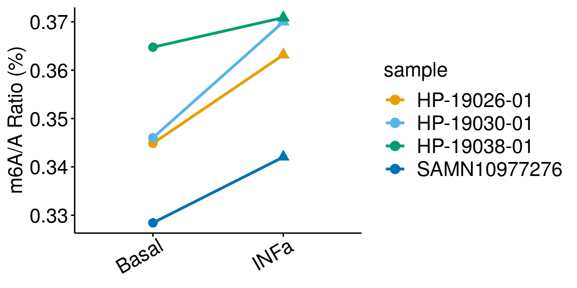
| Version | Author | Date |
|---|---|---|
| ce13e24 | scottzijiezhang | 2020-08-13 |
DT::datatable( compare_means(m6AvsA ~ condition, data = basalINa,
               paired = TRUE, method = "t.test"), rownames = FALSE )
basalILb <- dplyr::filter(all_m6A_new, condition %in% c("Basal","IL1b") )
ggplot(data = basalILb, mapping = aes( x= condition, y = m6AvsA*100 , color = sample, shape = condition, group = sample ) )+geom_line( size = 1)+geom_point( size = 3 )+
ylab("m6A/A Ratio (%)")+
theme_bw() + xlab("Condition")+theme(axis.ticks = element_line(color = "black"), panel.border = element_blank(),
panel.grid.minor = element_blank(), axis.line = element_line(colour = "black"), axis.text.x = element_text( size = 15, colour = "black",hjust = 0.9, angle = 30 ),axis.text.y = element_text( size =15, color = "black"),axis.title.x = element_blank(), axis.title.y = element_text( size =15), panel.grid = element_blank(), legend.text = element_text(size = 15), legend.title = element_text(size = 15) )+scale_color_manual(values = cbbPalette[-c(4)] )+scale_shape_discrete(guide = FALSE)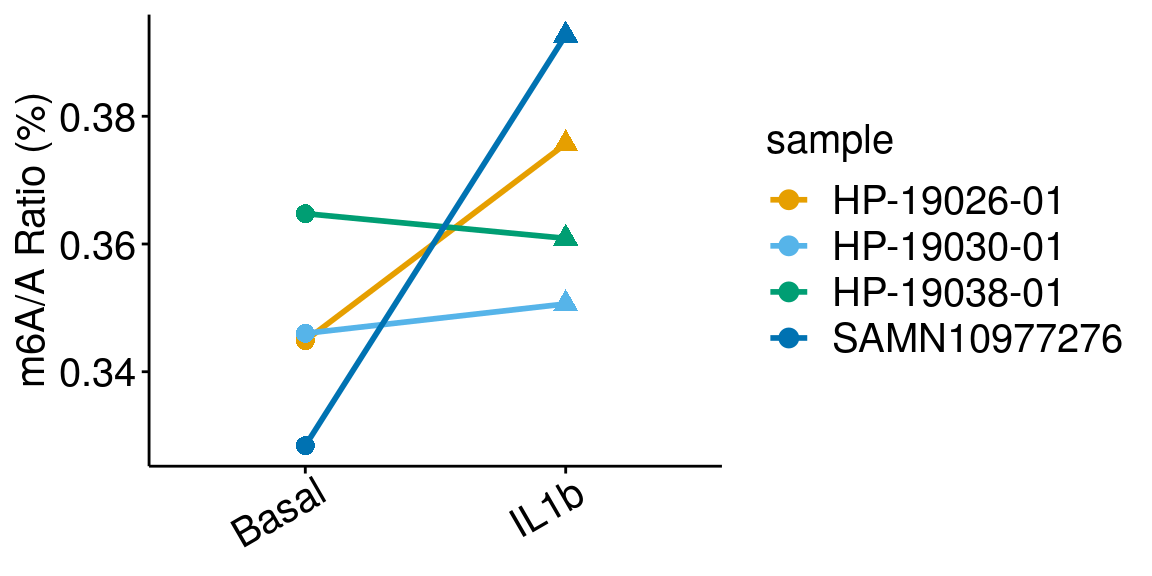
| Version | Author | Date |
|---|---|---|
| ce13e24 | scottzijiezhang | 2020-08-13 |
DT::datatable( compare_means(m6AvsA ~ condition, data = basalILb,
               paired = TRUE, method = "t.test"), rownames = FALSE )
basalTNFa <- dplyr::filter(all_m6A_new, condition %in% c("Basal","TNFa") )
ggplot(data = basalTNFa, mapping = aes( x= condition, y = m6AvsA*100 , color = sample, shape = condition, group = sample ) )+geom_line( size = 1)+geom_point( size = 3 )+
ylab("m6A/A Ratio (%)")+
theme_bw() + xlab("Condition")+theme(axis.ticks = element_line(color = "black"), panel.border = element_blank(),
panel.grid.minor = element_blank(), axis.line = element_line(colour = "black"), axis.text.x = element_text( size = 15, colour = "black",hjust = 0.9, angle = 30 ),axis.text.y = element_text( size =15, color = "black"),axis.title.x = element_blank(), axis.title.y = element_text( size =15), panel.grid = element_blank(), legend.text = element_text(size = 15), legend.title = element_text(size = 15) )+scale_color_manual(values = cbbPalette[-c(4)] )+scale_shape_discrete(guide = FALSE)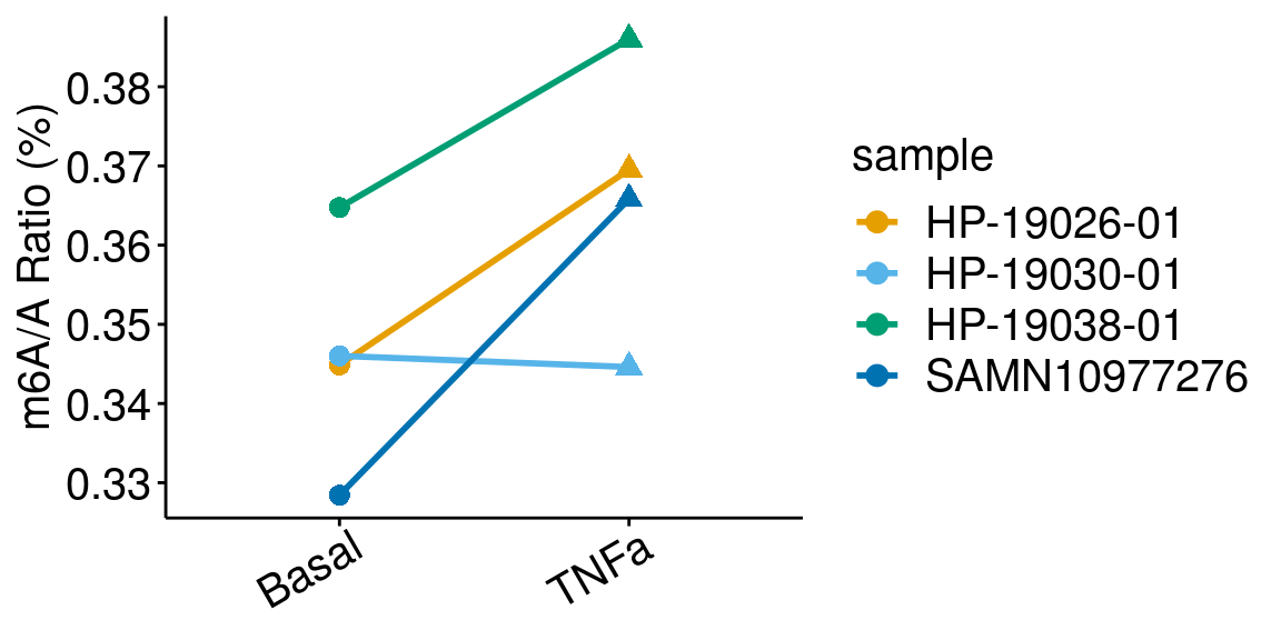
| Version | Author | Date |
|---|---|---|
| ce13e24 | scottzijiezhang | 2020-08-13 |
DT::datatable( compare_means(m6AvsA ~ condition, data = basalTNFa,
               paired = TRUE, method = "t.test"), rownames = FALSE )
basalGlucose <- dplyr::filter(all_m6A_new, condition %in% c("Basal","Glucose 19mM") )
ggplot(data = basalGlucose, mapping = aes( x= condition, y = m6AvsA*100 , color = sample, shape = condition, group = sample ) )+geom_line( size = 1)+geom_point( size = 3 )+
ylab("m6A/A Ratio (%)")+
theme_bw() + xlab("Condition")+theme(axis.ticks = element_line(color = "black"), panel.border = element_blank(),
panel.grid.minor = element_blank(), axis.line = element_line(colour = "black"), axis.text.x = element_text( size = 15, colour = "black",hjust = 0.9, angle = 30 ),axis.text.y = element_text( size =15, color = "black"),axis.title.x = element_blank(), axis.title.y = element_text( size =15), panel.grid = element_blank(), legend.text = element_text(size = 15), legend.title = element_text(size = 15) )+scale_color_manual(values = cbbPalette[-c(4)] )+scale_shape_discrete(guide = FALSE)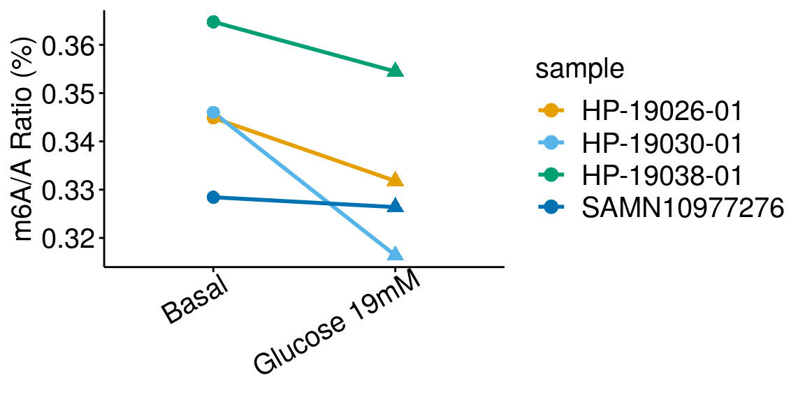
DT::datatable( compare_means(m6AvsA ~ condition, data = basalGlucose,
               paired = TRUE, method = "t.test"), rownames = FALSE )
basalPalmitate <- dplyr::filter(all_m6A_new, condition %in% c("Basal","Palmitate 500uM") )
ggplot(data = basalPalmitate, mapping = aes( x= condition, y = m6AvsA*100 , color = sample, shape = condition, group = sample ) )+geom_line( size = 1)+geom_point( size = 3 )+
ylab("m6A/A Ratio (%)")+
theme_bw() + xlab("Condition")+theme(axis.ticks = element_line(color = "black"), panel.border = element_blank(),
panel.grid.minor = element_blank(), axis.line = element_line(colour = "black"), axis.text.x = element_text( size = 15, colour = "black",hjust = 0.9, angle = 30 ),axis.text.y = element_text( size =15, color = "black"),axis.title.x = element_blank(), axis.title.y = element_text( size =15), panel.grid = element_blank(), legend.text = element_text(size = 15), legend.title = element_text(size = 15) )+scale_color_manual(values = cbbPalette[-c(4)] )+scale_shape_discrete(guide = FALSE)
DT::datatable( compare_means(m6AvsA ~ condition, data = basalPalmitate,
               paired = TRUE, method = "t.test"), rownames = FALSE )
sessionInfo()R version 3.5.3 (2019-03-11)
Platform: x86_64-pc-linux-gnu (64-bit)
Running under: Ubuntu 17.10
Matrix products: default
BLAS: /usr/lib/x86_64-linux-gnu/openblas/libblas.so.3
LAPACK: /usr/lib/x86_64-linux-gnu/libopenblasp-r0.2.20.so
locale:
[1] LC_CTYPE=en_US.UTF-8 LC_NUMERIC=C
[3] LC_TIME=en_US.UTF-8 LC_COLLATE=en_US.UTF-8
[5] LC_MONETARY=en_US.UTF-8 LC_MESSAGES=en_US.UTF-8
[7] LC_PAPER=en_US.UTF-8 LC_NAME=C
[9] LC_ADDRESS=C LC_TELEPHONE=C
[11] LC_MEASUREMENT=en_US.UTF-8 LC_IDENTIFICATION=C
attached base packages:
[1] stats graphics grDevices utils datasets methods base
other attached packages:
[1] ggsci_2.9 ggpubr_0.2 magrittr_1.5 ggplot2_3.1.1
loaded via a namespace (and not attached):
[1] Rcpp_1.0.1 later_0.8.0 compiler_3.5.3 pillar_1.3.1
[5] git2r_0.25.2 plyr_1.8.4 workflowr_1.3.0 tools_3.5.3
[9] digest_0.6.18 jsonlite_1.6 evaluate_0.13 tibble_2.1.1
[13] gtable_0.3.0 pkgconfig_2.0.2 rlang_0.4.0 shiny_1.3.2
[17] crosstalk_1.0.0 yaml_2.2.0 xfun_0.6 withr_2.1.2
[21] stringr_1.4.0 dplyr_0.8.0.1 knitr_1.22 fs_1.3.0
[25] htmlwidgets_1.3 rprojroot_1.3-2 grid_3.5.3 DT_0.5.1
[29] tidyselect_0.2.5 glue_1.3.1 R6_2.4.0 rmarkdown_1.12
[33] tidyr_0.8.3 purrr_0.3.2 whisker_0.3-2 promises_1.0.1
[37] backports_1.1.4 scales_1.0.0 htmltools_0.3.6 assertthat_0.2.1
[41] xtable_1.8-4 mime_0.6 colorspace_1.4-1 httpuv_1.5.1
[45] labeling_0.3 stringi_1.4.3 lazyeval_0.2.2 munsell_0.5.0
[49] crayon_1.3.4