Analyzing MeRIP-seq data with RADAR
Zijie Zhang, Chuan He, Mengjie Chen
6 February 2020
Abstract
A basic task in the analysis of MeRIP-seq is the detection of differentially methylated loci on the RNA. To analyze the count data of MeRIP-seq, we divide the transcript (concatenated exons of a gene) into consecutive bins and quantify the reads align to each bin. The summarized count data is in matrix format where each row represent a locus and each column is a sample. Statistical inference of changes across group, as compared to within-group variability was made for each filtered bin with sufficient count. This vignette explains the use of the package RADAR with example data. RADAR package version: 0.2.1
Note: if you use RADAR in published research, please cite:
Other packages with similar aims are exomePeak, MeTDiff, QNB.
1.Quick start
Here we show the most basic steps for a differential methylation analysis. There is one major step upstream of RADAR that generates mapped reads in BAM file for each sample, which can be done by varies choices of softwares such as Hisat2, tophat2 or Kallisto. we will discuss in the sections below assuming BAM file has been obtained.
This code chunk assumes that you have bam files for sample1-6 s1.input.bam, …, s6..input.bam and s1.m6A.bam, …, s6..m6A.bam and a vector of experimental group c("Ctl","Ctl","Ctl","Treated","Treated","Treated").
library(RADAR)
radar <- countReads(
  samplenames = c("s1","s2","s3","s4","s5","s6"),
  gtf = "/path/to/file.gtf",
  bamFolder = "/path/to/bam files",
  modification = "m6A",
  strandToKeep = "opposite",
  threads = 10
)

radar <- normalizeLibrary( radar )
radar <- adjustExprLevel( radar )
variable(radar) <- data.frame( group = c("Ctl","Ctl","Ctl","Treated","Treated","Treated") )
radar <- filterBins( radar ,minCountsCutOff = 15)
radar <- diffIP(radar)
## if using linux or mac, you can also use multi-thread mode
radar <- diffIP_parallel(radar)
radar <- reportResult( radar, cutoff = 0.1, Beta_cutoff = 0.5 )

res <- results( radar )
2.How to get help for
Issues and questions about the package should be posted to the issue report page of the github. The issue discussed here can be served as public knowledge base.
3.Standard workflow
a). Mapped BAM file.
To analyze for MeRIP-seq data, RADAR expect a pair of BAM file for each sample. For each pair of BAM file, the naming convention for RADAR is sample.input.bam for INPUT and sample.<methylation name>.bam for the IP, e.g. sample.m6A.bam for m6A IP sample. They key is INPUT and IP sample have the same prefix.
b). GTF annotation file.
For the organism being analyzed, user need to provide an annotation file in gtf format to define the genomic coordinate of gene features. A good source to download those supporting files are iGenome.
c). The MeRIP.RADAR object
The MeRIP and MeRIP.RADAR object are used by the RADAR package to store the intermediate data generated in the MeRIP-seq data pipeline. Please see Manul page for details.
d). Read count quantification.
We will use a toy data set to demonstrate how to start from bam file to count reads in consecutive bins and construct a RADAR dataset. There are 9 contols and 8 cases sample in the toy dataset. We name them by Ctl# and Case# in the following demonstrations.
library(RADAR)
samplenames <- c( paste0("Ctl",1:9), paste0("Case",1:8) )
Please note that user should set bam_dir to directory where bam files are saved in practice instead of setting it to package assocated example file folder system.file("extdata",package = "RADAR") in this example.
bam_dir <- system.file('extdata',package = 'RADAR')
samplenames
## [1] "Ctl1" "Ctl2" "Ctl3" "Ctl4" "Ctl5" "Ctl6" "Ctl7" "Ctl8"
## [9] "Ctl9" "Case1" "Case2" "Case3" "Case4" "Case5" "Case6" "Case7"
## [17] "Case8"Here we created a character vector samplenames to define the names of sample, which will later tells RADAR to look for input and IP file with the samplenames as prefix.
Next we need to use countReads() function to 1) concatenate exons of each gene to get a “longest isoform” transcript of each gene. 2) Divide transcripts into consecutive bins of user defined width. 3) quantify reads mapped to each bin.
This step usually takes a few hours depending on the configuration of the computer and the number of thread used to count reads. In a workstation using 20 threads (Intel Xeon processer), it takes about 1 hour for this step for 15 samples. Much longer time is expected if using laptop.
note 1 The parameter modification = "m6A" tells the function to look for bam file of IP by the name samplename.m6A.bam. If the user named the IP sample as samplename.IP.bam, the user should set modification = "IP". We enable flexible seeting for IP sample in cases where user perform MeRIP seq on multiple modification with shared INPUT library.
note 2 In Linux or MacOs, our package support multi-thread mode enabled by R package doParallel . One can set the number of threads to use by threads = n. note 3 The default setting for bin width to slice the transcript is 50bp. One can set this by parameter binSize = #bp. For very shallow sequencing depth (e.g. less than 10M mappable reads per library), we recommand setting bin width to larger size such as 100bp to increase the number of reads countable in each bin.
note 4 The parameter fragmentLength defines the number of nucleotide to shift from the head of a read in BAM record to the center of RNA fragment. In the example data, the RNA has been sonicated into ~150nt fragment before IP and library preparation.
radar <- countReads(samplenames = samplenames,
                    gtf = "~/Database/genome/hg38/hg38_UCSC.gtf",
                    bamFolder = bam_dir,
                    modification = "m6A",
                    fragmentLength = 150,
                    outputDir = "test",
                    threads = 20,
                    binSize = 50
)
## [1] "Stage: index bam file /home/zijiezhang/R/x86_64-pc-linux-gnu-library/3.5/RADAR/extdata/Ctl1.input.bam"
## [1] "Stage: index bam file /home/zijiezhang/R/x86_64-pc-linux-gnu-library/3.5/RADAR/extdata/Ctl1.m6A.bam"
## [1] "Stage: index bam file /home/zijiezhang/R/x86_64-pc-linux-gnu-library/3.5/RADAR/extdata/Ctl2.input.bam"
## [1] "Stage: index bam file /home/zijiezhang/R/x86_64-pc-linux-gnu-library/3.5/RADAR/extdata/Ctl2.m6A.bam"
## [1] "Stage: index bam file /home/zijiezhang/R/x86_64-pc-linux-gnu-library/3.5/RADAR/extdata/Ctl3.input.bam"
## [1] "Stage: index bam file /home/zijiezhang/R/x86_64-pc-linux-gnu-library/3.5/RADAR/extdata/Ctl3.m6A.bam"
## [1] "Stage: index bam file /home/zijiezhang/R/x86_64-pc-linux-gnu-library/3.5/RADAR/extdata/Ctl4.input.bam"
## [1] "Stage: index bam file /home/zijiezhang/R/x86_64-pc-linux-gnu-library/3.5/RADAR/extdata/Ctl4.m6A.bam"
## [1] "Stage: index bam file /home/zijiezhang/R/x86_64-pc-linux-gnu-library/3.5/RADAR/extdata/Ctl5.input.bam"
## [1] "Stage: index bam file /home/zijiezhang/R/x86_64-pc-linux-gnu-library/3.5/RADAR/extdata/Ctl5.m6A.bam"
## [1] "Stage: index bam file /home/zijiezhang/R/x86_64-pc-linux-gnu-library/3.5/RADAR/extdata/Ctl6.input.bam"
## [1] "Stage: index bam file /home/zijiezhang/R/x86_64-pc-linux-gnu-library/3.5/RADAR/extdata/Ctl6.m6A.bam"
## [1] "Stage: index bam file /home/zijiezhang/R/x86_64-pc-linux-gnu-library/3.5/RADAR/extdata/Ctl7.input.bam"
## [1] "Stage: index bam file /home/zijiezhang/R/x86_64-pc-linux-gnu-library/3.5/RADAR/extdata/Ctl7.m6A.bam"
## [1] "Stage: index bam file /home/zijiezhang/R/x86_64-pc-linux-gnu-library/3.5/RADAR/extdata/Ctl8.input.bam"
## [1] "Stage: index bam file /home/zijiezhang/R/x86_64-pc-linux-gnu-library/3.5/RADAR/extdata/Ctl8.m6A.bam"
## [1] "Stage: index bam file /home/zijiezhang/R/x86_64-pc-linux-gnu-library/3.5/RADAR/extdata/Ctl9.input.bam"
## [1] "Stage: index bam file /home/zijiezhang/R/x86_64-pc-linux-gnu-library/3.5/RADAR/extdata/Ctl9.m6A.bam"
## [1] "Stage: index bam file /home/zijiezhang/R/x86_64-pc-linux-gnu-library/3.5/RADAR/extdata/Case1.input.bam"
## [1] "Stage: index bam file /home/zijiezhang/R/x86_64-pc-linux-gnu-library/3.5/RADAR/extdata/Case1.m6A.bam"
## [1] "Stage: index bam file /home/zijiezhang/R/x86_64-pc-linux-gnu-library/3.5/RADAR/extdata/Case2.input.bam"
## [1] "Stage: index bam file /home/zijiezhang/R/x86_64-pc-linux-gnu-library/3.5/RADAR/extdata/Case2.m6A.bam"
## [1] "Stage: index bam file /home/zijiezhang/R/x86_64-pc-linux-gnu-library/3.5/RADAR/extdata/Case3.input.bam"
## [1] "Stage: index bam file /home/zijiezhang/R/x86_64-pc-linux-gnu-library/3.5/RADAR/extdata/Case3.m6A.bam"
## [1] "Stage: index bam file /home/zijiezhang/R/x86_64-pc-linux-gnu-library/3.5/RADAR/extdata/Case4.input.bam"
## [1] "Stage: index bam file /home/zijiezhang/R/x86_64-pc-linux-gnu-library/3.5/RADAR/extdata/Case4.m6A.bam"
## [1] "Stage: index bam file /home/zijiezhang/R/x86_64-pc-linux-gnu-library/3.5/RADAR/extdata/Case5.input.bam"
## [1] "Stage: index bam file /home/zijiezhang/R/x86_64-pc-linux-gnu-library/3.5/RADAR/extdata/Case5.m6A.bam"
## [1] "Stage: index bam file /home/zijiezhang/R/x86_64-pc-linux-gnu-library/3.5/RADAR/extdata/Case6.input.bam"
## [1] "Stage: index bam file /home/zijiezhang/R/x86_64-pc-linux-gnu-library/3.5/RADAR/extdata/Case6.m6A.bam"
## [1] "Stage: index bam file /home/zijiezhang/R/x86_64-pc-linux-gnu-library/3.5/RADAR/extdata/Case7.input.bam"
## [1] "Stage: index bam file /home/zijiezhang/R/x86_64-pc-linux-gnu-library/3.5/RADAR/extdata/Case7.m6A.bam"
## [1] "Stage: index bam file /home/zijiezhang/R/x86_64-pc-linux-gnu-library/3.5/RADAR/extdata/Case8.input.bam"
## [1] "Stage: index bam file /home/zijiezhang/R/x86_64-pc-linux-gnu-library/3.5/RADAR/extdata/Case8.m6A.bam"
## Reading gtf file to obtain gene model
## Filter out ambiguous model...
## Gene model obtained from gtf file...
## counting reads for each genes, this step may takes a few hours....
## Hyper-thread registered: TRUE
## Using 20 thread(s) to count reads in continuous bins...
## Time used to count reads: 17.3461465080579 mins...This function returns a MeRIP object that stores the read counts in consecutive bin. We can check the summary of this MeRIP object by:
summary(radar)## MeRIP dataset of 17 samples.
## Read count quantified in 50-bp consecutive bins on the transcript.
## The total read count for Input and IP samples are (Million reads):
## Ctl1 Ctl2 Ctl3 Ctl4 Ctl5 Ctl6 Ctl7 Ctl8 Ctl9 Case1 Case2 Case3 Case4
## Input 0.08 0.09 0.08 0.07 0.04 0.06 0.08 0.08 0.08 0.08 0.08 0.06 0.09
## IP 0.13 0.10 0.09 0.05 0.06 0.07 0.13 0.10 0.10 0.11 0.11 0.10 0.10
## Case5 Case6 Case7 Case8
## Input 0.05 0.07 0.10 0.08
## IP 0.13 0.09 0.09 0.09More information about MeRIP object and the data slots in this object can be found in the Manul page.
e). Pre-processing the read count data.
After obtaining the radar object containing read count, we can then proceed to library normalization step.
This step should takes a few minutes.
radar <- normalizeLibrary(radar)
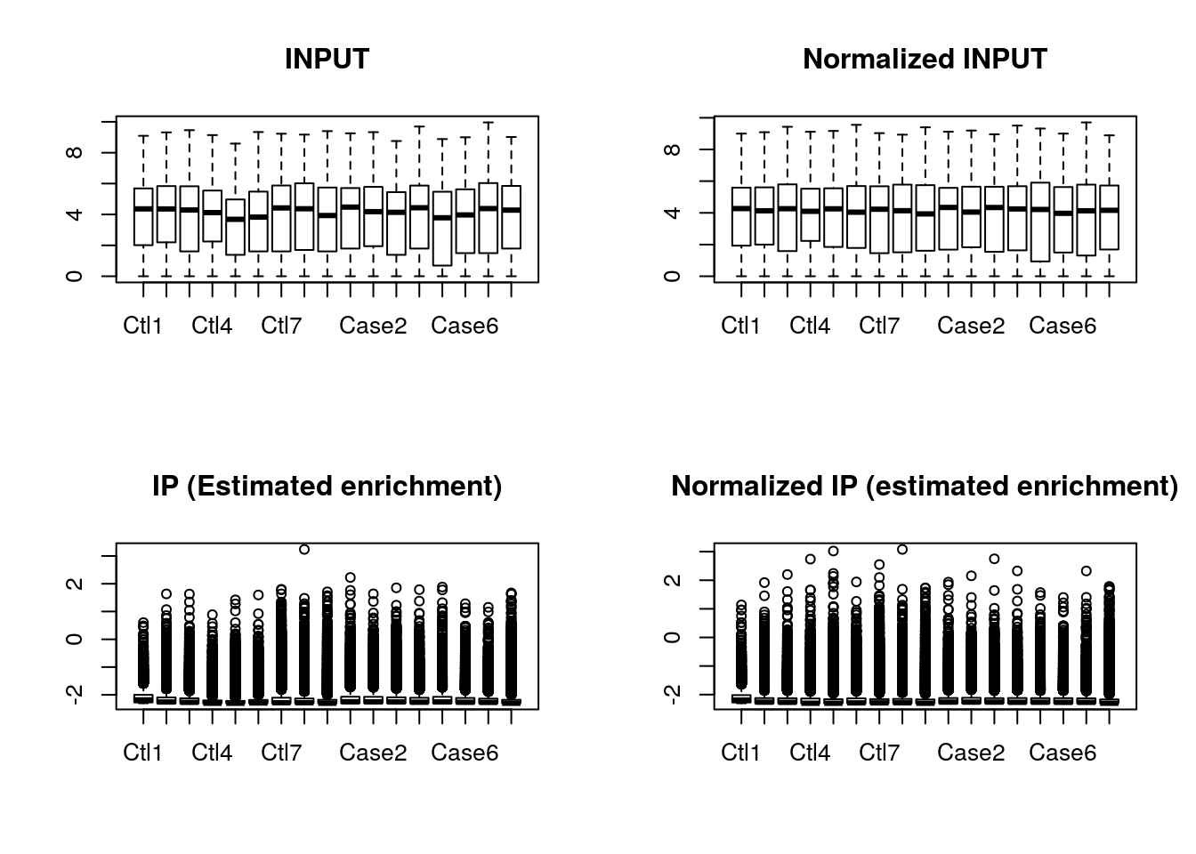
In this step, the bin-level read count of input is summarized into gene-level read count. The size factor of input is calculated using “mean ratio method” implemented in DESeq2, which is then used to calculated normalized input bin-level read count. To normalize the library size of IP samples, we use top read count bins of IP and corresponding input gene-level read count to compute the estimated enrichment of each sample. This procedure is under the assumption that samples in the same study have the same IP efficiency. We then normalize the IP read counts by the estimated IP efficiency. As an sanity check, in addition to return the radar object with normalized read count, the normalizeLibrary() function also generate box plot of read count before and after normalizing INPUT and box plot of estimated enrichment before and after normalizing IP. This plot can be disabled by option boxPlot = FALSE.
This function will return a MeRIP.RADAR object. There will be normalized gene-level INPUT count matrix stored in this object, which is essentially RNA-seq read count matrix and can be accessed by geneExression(radar). The normalized bin-level read count matrix will be also stored. The MeRIP.RADAR object will also contain size factor sizeFactors(radar) used to normalize each library.
sizeFactors(radar)## input ip
## Ctl1 1.0979767 1.0914554
## Ctl2 1.2570283 1.2001060
## Ctl3 1.0292293 1.0239868
## Ctl4 1.0232009 0.5961540
## Ctl5 0.5603525 0.6036450
## Ctl6 0.8057010 0.7040740
## Ctl7 1.2196053 1.4418411
## Ctl8 1.2674578 1.1722820
## Ctl9 0.9987106 0.9866003
## Case1 1.1456290 1.3452576
## Case2 1.1448646 1.2761950
## Case3 0.8185538 1.2392203
## Case4 1.2087343 1.1124690
## Case5 0.6464346 1.3732866
## Case6 1.0002226 1.0764286
## Case7 1.2894405 0.9766605
## Case8 1.1322811 0.9677948Next, we can use the geneSum of INPUT to adjust for the variation of expression level of the IP read count. This step aims to account for the variation of IP read count attributed to variation of pre-IP gene expression level.
radar <- adjustExprLevel(radar)## Adjusting expression level using Input geneSum read count...If you expect intensive alternative splicing events cross the experimental groups, using gene-level read counts to represent pre-IP RNA level could leads to bias. Therefore, the user can also choose to use the local bin-level read count to adjust the pre-IP RNA level variation:
radar <- adjustExprLevel(radar, adjustBy = "pos")Next, we will need to filter out bins of very low read count because under sampled locus can be strongly affected by technical variation. This step will also filter out bins where IP has less coverage than Input because we only care about loci where m6A is enrichment.
Beside, we will also need to provide the experimental group to the MeRIP.RADAR object for filtering and later inferential test steps.
variable(radar) <- data.frame( Group = c(rep("Ctl",9),rep("Case",8)) )

radar <- filterBins(radar,minCountsCutOff = 15)
## Filtering bins with low read counts...
## Bins with average counts lower than 15 in both groups have been removed...
## Filtering bins that is enriched in IP experiment...e). Run Poisson Gamma Test
Now we have the pre-processed read counts matrix for testing differential methylation. To run the default PoissonGamma test, we can call the diiIP() function:
radar <- diffIP(radar)Depending on the number of bins to be processed, this step may takes minutes to hours. Thus, multi-thread is recommended.
radar <- diffIP_parallel(radar, thread = 8)The code above run test on the effect of predictor variable on the methylation level, which is fine if all covariates are well balanced. However, in most cases, samples might have been processed in more than one batches (especially when sample size is large) where batch effect and other covariate could contributed to the variation.
f). PCA analysis
In order to check for unwanted variation, we can take the top 1000 bins ranked by count number (basically using the high read count bins) to plot PCA:
top_bins <- extractIP(radar,filtered = T)[order(rowMeans( extractIP(radar,filtered = T) ),decreasing = T)[1:1000],]## Returning normalized IP read counts.
## Returning normalized IP read counts.plotPCAfromMatrix(top_bins,group = unlist(variable(radar)) )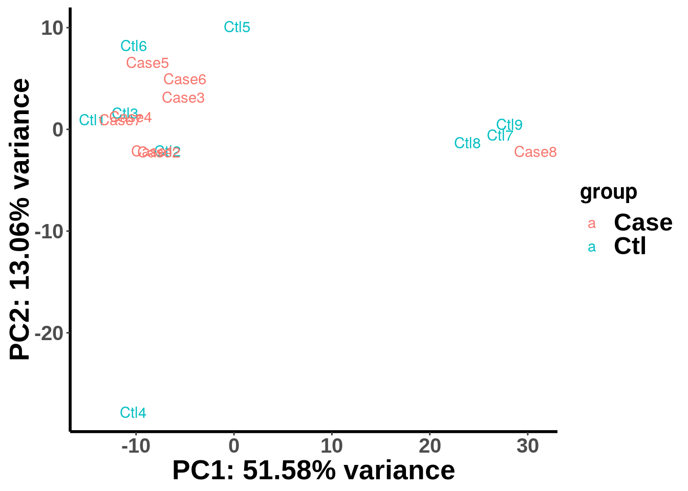
We can see that our Case and Control are not well separated by the first two PCs. To check if the samples are separated by batches, we can label the samples by batch instead of by experimental group X.
batch <- c("A","A","A","A","B","B","C","C","C","A","A","B","A","B","B","A","C")
plotPCAfromMatrix(top_bins,group = batch)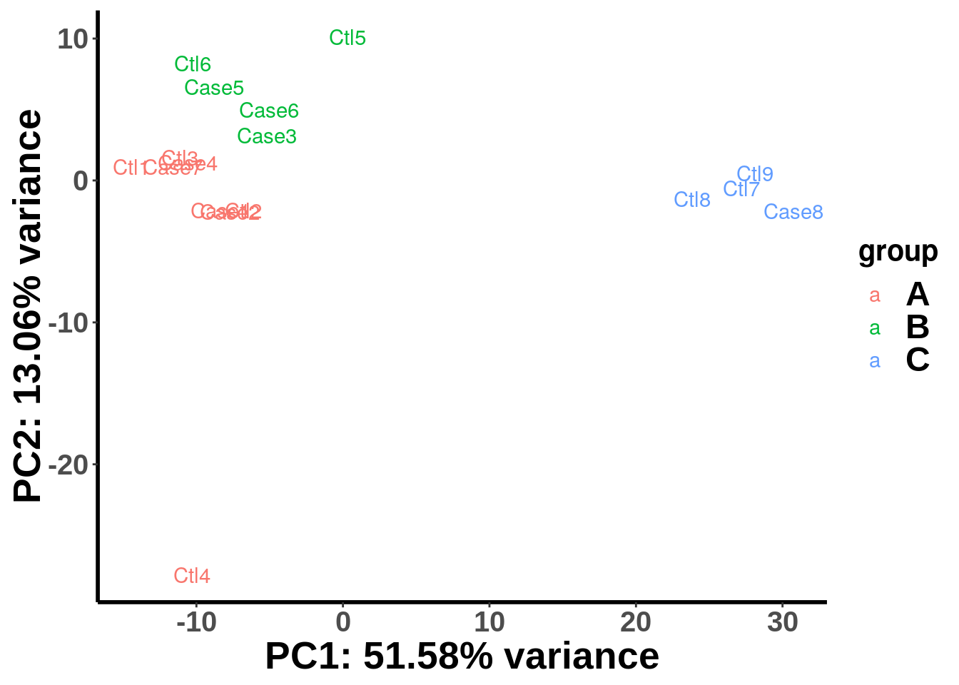
We can see that the samples are clearly separated by batches and we need to account for batch effect in the test. To incorporate covariates in study design, we need first define a covariate matrix table where categorical variable should be converted to (0,1) binary variable.
library(rafalib)
X2 <- as.fumeric(c("A","A","A","A","B","B","A","A","A","A","A","B","A","B","B","A","A"))-1 # batch as covariates
X3 <- as.fumeric(c("A","A","A","A","A","A","C","C","C","A","A","A","A","A","A","A","C"))-1 # batch as covariates
X4 <- as.fumeric(c("M","M","F","M","M","M","F","M","M","M","M","F","M","M","M","M","F"))-1 # sex as covariates
cov <- cbind(X2,X3,X4)

## set the new variable with covariates
variable(radar) <- cbind(variable(radar), cov)
Run the Poisson Gamma test with covariates to account for know source of variation.
radar <- diffIP(radar)or multithread mode
## The predictor variable has been converted:
##  Ctl  Ctl  Ctl  Ctl  Ctl  Ctl  Ctl  Ctl  Ctl Case Case Case Case Case Case
##    0    0    0    0    0    0    0    0    0    1    1    1    1    1    1
## Case Case
##    1    1
## running PoissonGamma test at multi-beta mode...
## Hyper-thread registered: TRUE
## Using 10 thread(s) to run multi-beta PoissonGamma test...
## Time used to run multi-beta PoissonGamma test: 0.018441383043925 mins...
If for some reasons you want to remove a few samples from the test, you can set index number of the samples you want to skip to exclude them in the Poisson Gamma test.
diffIP_parallel(radar, exclude = c("Ctl1","Ctl4") )In the radar object returned by the diffIP(), a mtrix of test statistics has been stored there.
To check the test statistics of the Poisson Gamma (random effect model) test, one can extract the estimators by:
head(radar@test.est)## psi mu2 beta beta2 beta3
## AHCYL1,75 9.678722 3.522843 -0.09641892 0.28414582 -0.9420370
## AHCYL1,124 6.066773 3.967197 -0.37917505 0.78421707 -1.0446384
## AHCYL1,174 13.508426 2.942321 -0.50132547 1.53579698 -0.3897320
## AHCYL1,224 35.793768 1.107990 -0.41389434 2.84375797 0.5871112
## AHCYL1,273 5.724238 3.112765 -0.36436277 1.44939833 -0.4613233
## AHCYL1,4844 7.040357 3.815238 -0.32912916 -0.03345433 -1.2758823
## beta4 SE1 SE2 SE3 SE4 SE5
## AHCYL1,75 -0.16447899 4.640891 0.1724507 0.1895064 0.2062545 0.2693174
## AHCYL1,124 -0.10603470 2.341075 0.2057603 0.2208556 0.2441250 0.3015791
## AHCYL1,174 0.03313673 10.312134 0.1629181 0.1838040 0.1978682 0.2613648
## AHCYL1,224 -0.08639388 48.380491 0.2453205 0.1966249 0.2552465 0.3523041
## AHCYL1,273 0.20837154 2.533215 0.1959419 0.2357435 0.2600130 0.3302250
## AHCYL1,4844 -0.18004743 2.955681 0.1733210 0.2200552 0.2433238 0.3106699
## SE6 p_value1 p_value2 p_value p_value4
## AHCYL1,75 0.2317938 0.037021150 9.406106e-93 0.610899608 1.683124e-01
## AHCYL1,124 0.2694532 0.009557306 7.805491e-83 0.086007289 1.316497e-03
## AHCYL1,174 0.2264891 0.190211253 6.567686e-73 0.006381609 8.378662e-15
## AHCYL1,224 0.2484970 0.459397769 6.286972e-06 0.035291761 7.902681e-29
## AHCYL1,273 0.2952550 0.023841520 7.901750e-57 0.122203629 2.484829e-08
## AHCYL1,4844 0.2784918 0.017220096 2.183117e-107 0.134740680 8.906443e-01
## p_value5 p_value6 likelihood fdr
## AHCYL1,75 4.689904e-04 0.4779574 -63.19130 0.9994913
## AHCYL1,124 5.324146e-04 0.6939369 -72.72130 0.5347707
## AHCYL1,174 1.359243e-01 0.8836798 -58.31225 0.1747750
## AHCYL1,224 9.561585e-02 0.7280913 -44.21530 0.3951978
## AHCYL1,273 1.624146e-01 0.4803535 -66.62640 0.6115589
## AHCYL1,4844 4.010482e-05 0.5179499 -64.84996 0.6307191Due to the resolution of the MeRIP-seq experiment where RNA molecules are fragmented into 100-300nt, neighboring bins can usually contain reads from the same locus. Therefore, we do a post-processing to merge significant neighboring bins after the test to obtain a final list of differential peaks. We merge the p-value of connecting bins by fisher’s method and report the max beta from neighbouring bins.
radar <- reportResult(radar, cutoff = 0.1, Beta_cutoff = 0.5)## Hyper-thread registered: TRUE
## Using 1 thread(s) to report merged report...
## Time used to report peaks: 0.0142485539118449 mins...
## When merging neighboring significant bins, logFC was reported as the max logFC among these bins.
## p-value of these bins were combined by Fisher's method.Here, we use FDR<0.1 and log fold change > 0.5 as default cutoff for selecting significant bins. Users can also specify these parameters by cutoff for FDR cutoff and Beta_cutoff for log fold change cutoff.
Finally, we can extract the final result as an table (in BED12 format) for the genomic location of the differential methylated peaks with p-values and log fold changes.
result <- results(radar)## There are 15 reported differential loci at FDR < 0.1 and logFoldChange > 0.5.head(result)## chr start end name score strand thickStart thickEnd
## 1 chr1 109625391 109625440 AMPD2 0 + 109625391 109625440
## 2 chr1 112653599 112653648 CAPZA1 0 + 112653599 112653648
## 3 chr1 117929480 117929529 GDAP2 0 - 117929480 117929529
## 4 chr1 110210963 110211012 KCNC4 0 + 110210963 110211012
## 5 chr1 110212010 110212059 KCNC4 0 + 110212010 110212059
## 6 chr1 109202989 109203038 KIAA1324 0 + 109202989 109203038
## itemRgb blockCount blockSizes blockStarts logFC p_value
## 1 0 1 49 0 -0.6156509 4.399273e-05
## 2 0 1 49 0 0.6198673 8.422996e-04
## 3 0 1 49 0 -0.5180336 1.025808e-03
## 4 0 1 49 0 -0.5713663 1.175029e-03
## 5 0 1 49 0 -0.7828979 1.233490e-05
## 6 0 1 49 0 -0.5611710 2.257110e-04g). Visualize the result by heatmap
To assess the pattern of variation of the MeRIP-seq data, we can plot the heatmap of methylation level (represented by the normalized IP read counts adjusted for expression level).
The belowing code shows how to plot heatmap from the MeRIP.RADAR object for the significant bins.
plotHeatMap(radar)## Plot heat map for differential loci at FDR < 0.1 and logFoldChange > 0.5.
## Returning normalized and expression level adjusted IP read counts.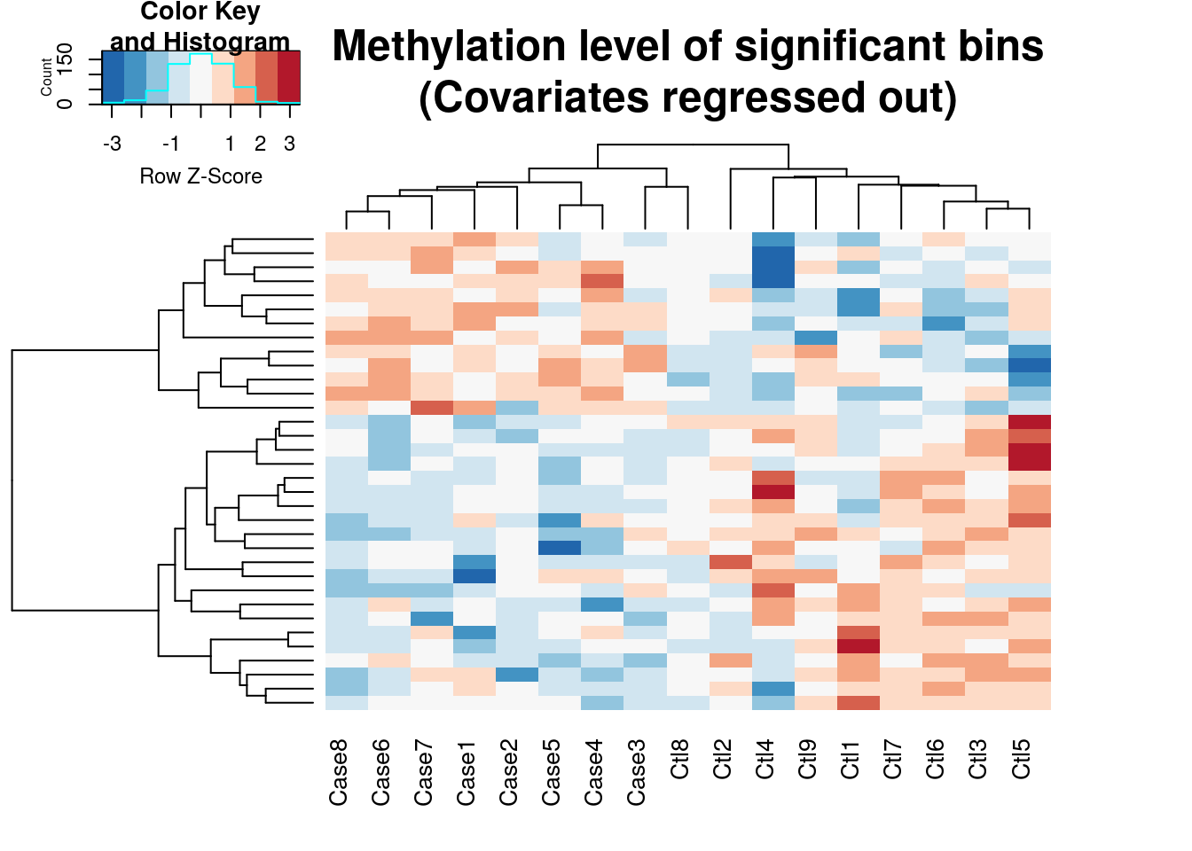
Note as we determined earlier by PCA plot, batch effect is contibuting substantially to the variability of our data set. By default plotHeatMap function regress out covariates when the number of columns of the variable(radar) > 1. If we want to see the heatmap before regressing out covariates, we can disable it by:
plotHeatMap(radar,covariates = FALSE)## Plot heat map for differential loci at FDR < 0.1 and logFoldChange > 0.5.
## Returning normalized and expression level adjusted IP read counts.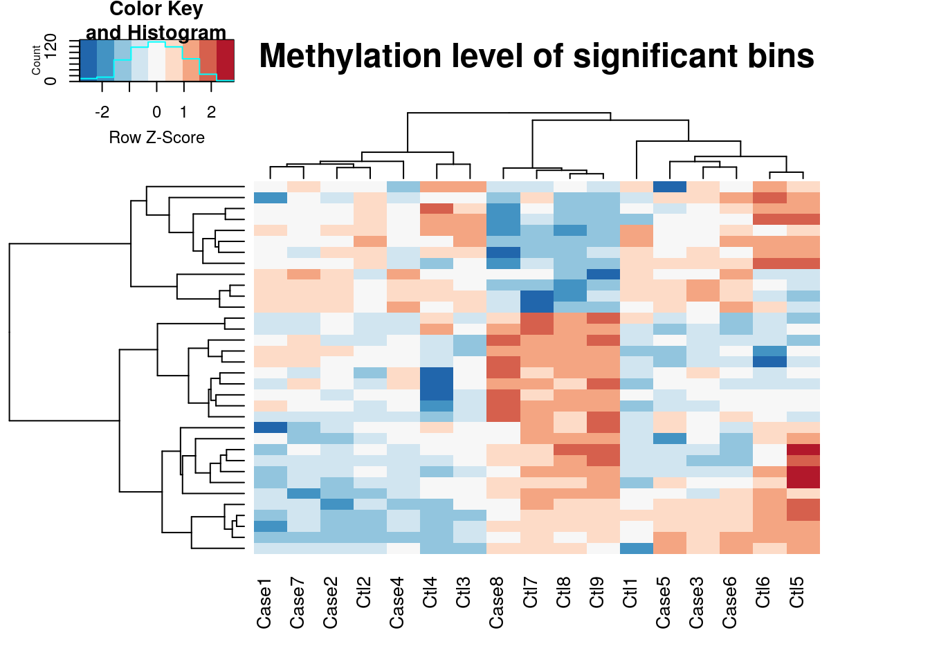
Since plotting too many bins willl look very messy, the function takes the top 5000 bins ranked by test p value. In another words, the heatmap generated here is a visualization the top differential methylated loci. From the heatmap we can see the methylation profile of Ctl8 looks much closer to Cases than to Controls, which suggest this sample is an outlier.
At this point, one can proceed to the next step to report the significantly differentially methylated bins to genomic location or repeat the analysis excluding the outlier sample.
h). Visualize MeRIP-seq data by sequencing coverage plot.
One of the most straight forward visualization of MeRIP-seq data is the coverage plot. We implemented function to take a radar object and plot the mean/median coverage of IP and INPUT for two inferential groups. Here we demonstrate the function using a differential methylated gene reported in above sections.
To use the plot function, we need to prepare an GTF annotation in GRanges format. This can be done by radar <- PrepCoveragePlot(radar). This step only need to be done once for each MeRIP.RADAR object.
radar <- PrepCoveragePlot(radar)
plotGeneCov(radar,geneName = "SLC25A24", center = median, libraryType = "opposite")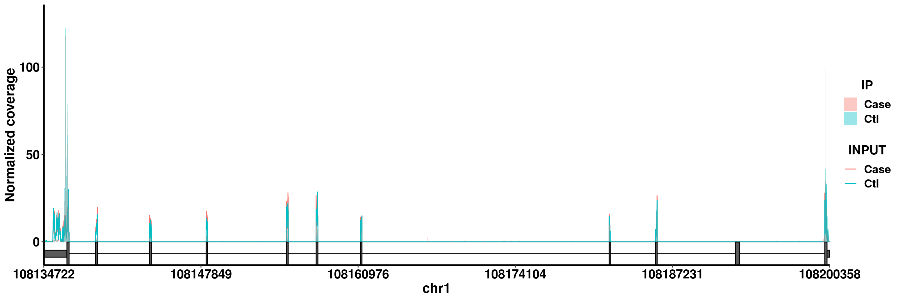
Note The parameter center = median defines how to combine replicates of the same group. You can also set it to be center = mean so that the coverage of each group is calculated by taking the mean of replicates.
In some cases, the gene has very long introns that the exon regions become too narrow to be clearly seen in the whole gene plot. We can call the same function with additional parameter ZoomIn to define a range in the gene to plot (Note ZoomIn range need to be within the gene).
plotGeneCov(radar,geneName = "SLC25A24", center = median, libraryType = "opposite",ZoomIn = c(108200059,108200308 ) )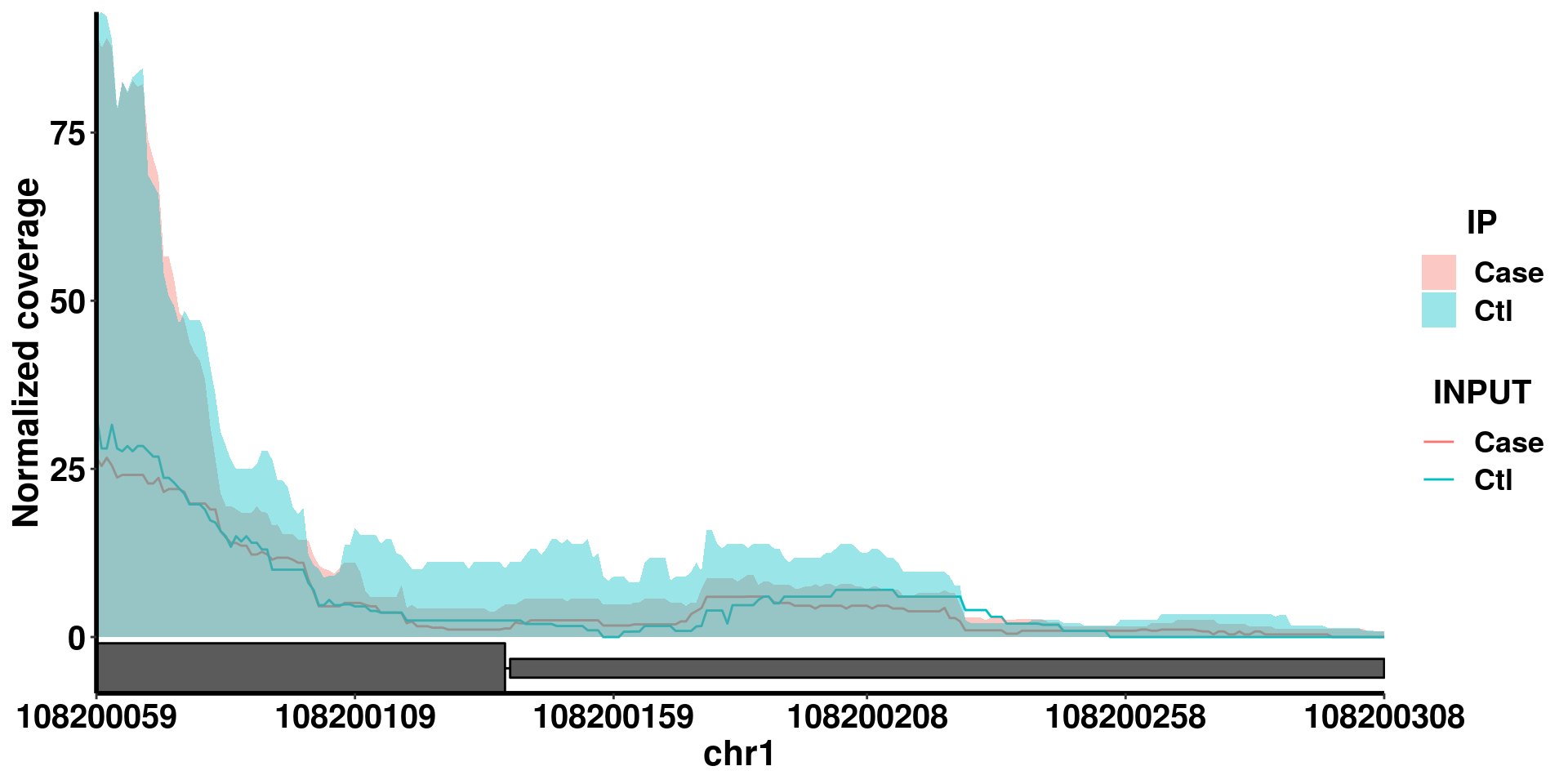
From the coverage plot we can see the in the “Case” group, the m6A peak is significantly decreased.
Another option of plotGeneCov is adjustExprLevel. To facilitate direct comparison of methylation level, we can choose to normalize the coverage by the gene expression level (input) so that the coverage of the IP is directly comparable between two groups.
plotGeneCov(radar,geneName = "SLC25A24", center = mean, libraryType = "opposite",ZoomIn = c(108200059,108200308 ), adjustExprLevel = T )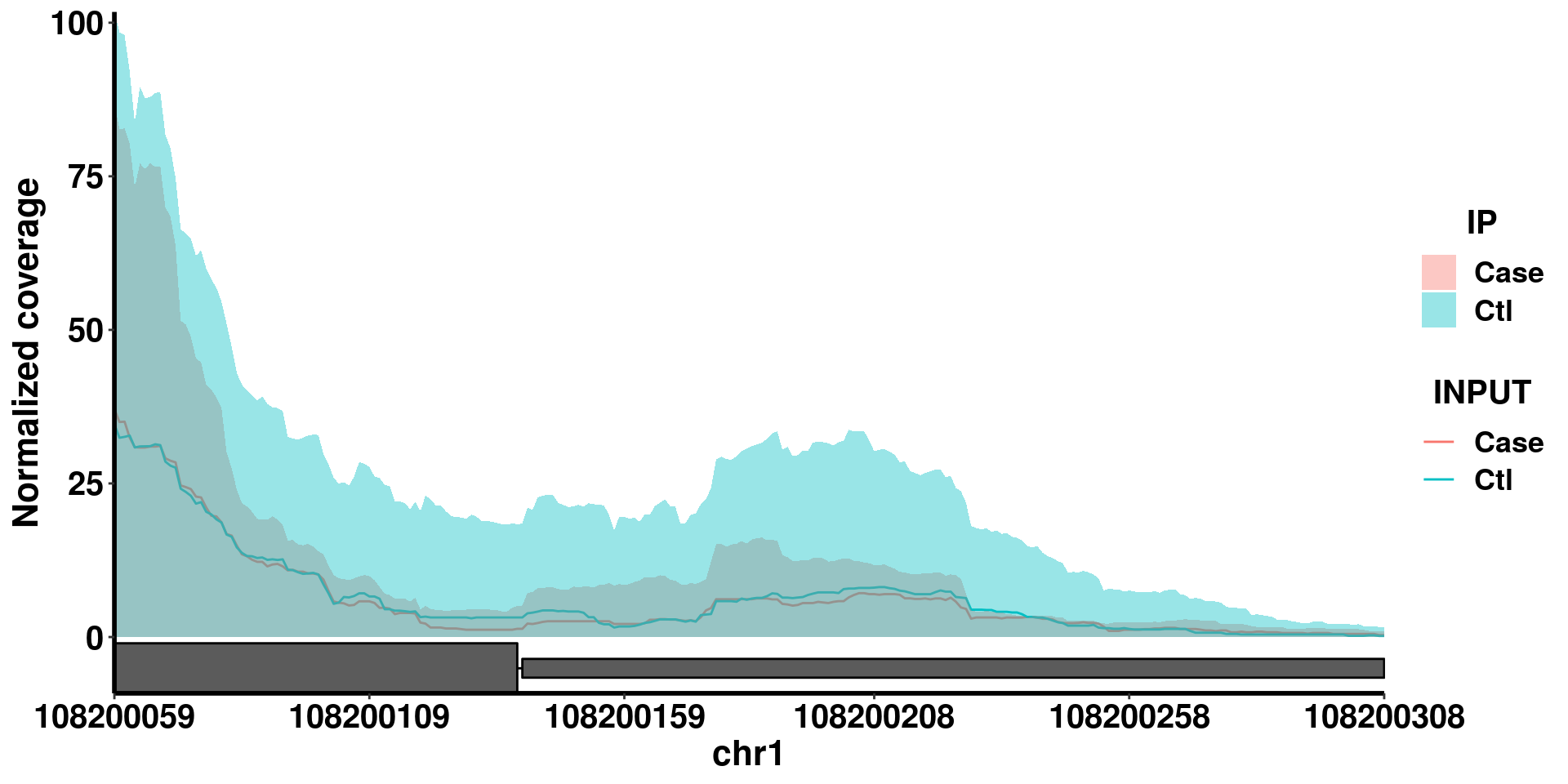 In this case, it doesn’t make much difference because the expression level of this gene is not differentially expressed. So it won’t be very different if we normalize all coverages by the expression level.
In some cases, user may want to check the variability of the methylation level among samples, which would not be captured by the mean coverage plot. So we can plot each individual sample in a panel to compare sample sample variations.
plotGeneCov(radar,geneName = "SLC25A24", libraryType = "opposite",ZoomIn = c(108200059,108200308 ), adjustExprLevel = T , split = T)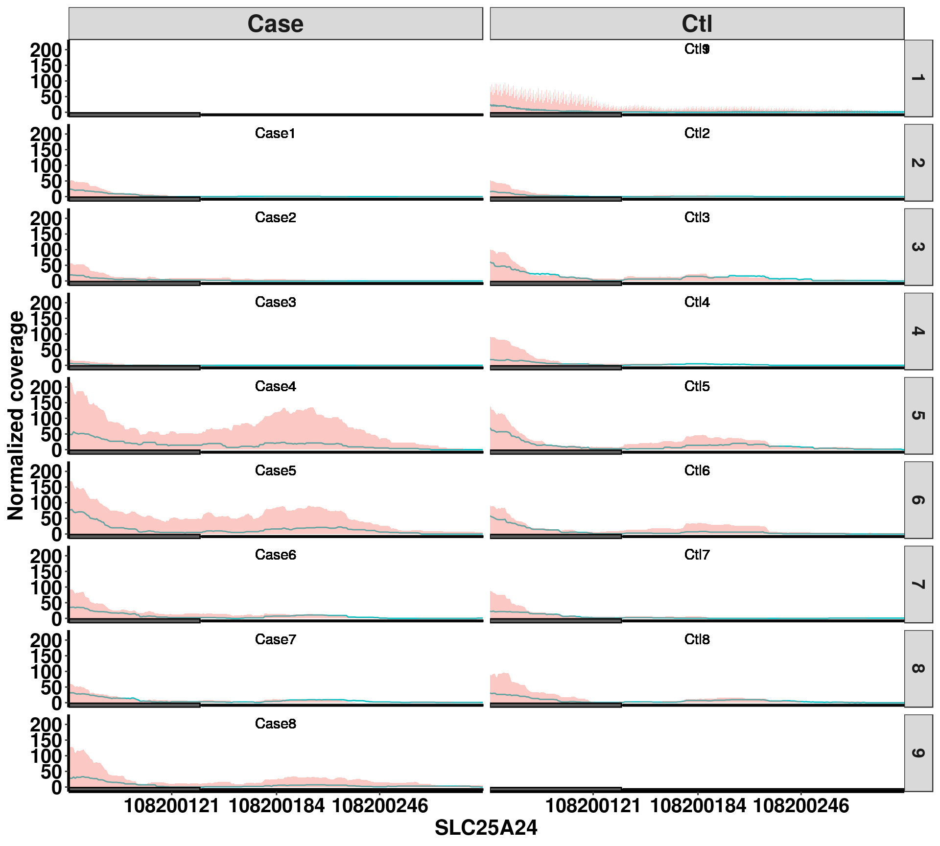
4. Model
a). Poisson model
\[\begin{eqnarray*} Y_{i} &\sim& Poi(\lambda_{i}) \\ \log(\lambda_{i} ) & = & \mu_1 + X_i \beta +e_{i} \end{eqnarray*}\] We assume random effect \(e_{i} \in \log\text{Gamma}(\psi, \psi)\), with scale parameter \(\psi\) and mean equal to \(1\). This is equivalent to \(\lambda_{i} = e^{ \mu_1 + X_i \beta} w_i\) where \(w_i \in \text{Gamma}(\psi, \psi)\) .\[\begin{eqnarray*} P( Y_i | \Theta, - w_i) &=& \int e^{-w_i e^{ \mu_1 + X_i \beta}} \frac{(w_i e^{ \mu_1 + X_i \beta} )^{Y_i}}{Y_i!} \frac{\psi^\psi w_i^{\psi-1}e^{-\psi w_i}}{\Gamma(\psi)} d w_i\\ &=& \frac{ \psi^\psi }{Y_i! } \frac{ \Gamma(Y_i+\psi) } {\Gamma(\psi) } \frac{ (e^{ \mu_1 + X_i \beta})^{Y_i}}{ (e^{ \mu_1 + X_i \beta} + \psi)^{Y_i + \psi}} \end{eqnarray*}\] The marginal log likelihood of observing \(\mathbf{Y}\) can be written as: \[\begin{eqnarray*} \log L( \mathbf{Y} ) &=& \sum_{i}^n [ Y_i( \mu_1 + X_i \beta) + \psi \log \psi + \log \Gamma(Y_i + \psi) - \log Y_i! - \log \Gamma( \psi) - (Y_i + \psi) \log( e^{ \mu_1 + X_i \beta} + \psi)] \\ \end{eqnarray*}\]
b). Estimation
We use gradient ascent algorithm to estimate the parameters, which involves the calculation of first derivatives.\[\begin{eqnarray*} \frac{ \partial \log L( \mathbf{Y} ) }{ \partial \beta } &=& \sum_{i}^n \ \Big[ Y_i - \big (Y_i + \psi \big )\frac{e^{ \mu_1+ X_i \beta}}{ e^{ \mu_1 + X_i \beta} +\psi} \Big] X_i \\ \frac{ \partial \log L( \mathbf{Y} ) }{ \partial \psi} &=& \sum_{i}^n \Big [ \log \psi + 1 - \frac{Y_i + \psi }{ e^{ \mu_1 + X_i \beta} +\psi} - \log ( e^{ \mu_1 + X_i \beta} +\psi ) \\ &&+ \text{digamma} ( Y_i + \psi) - \text{digamma} ( \psi) \Big ] \\ \frac{ \partial \log L( \mathbf{Y} ) }{ \partial \mu _1} &=& \sum_{i}^n \Big[ Y_i - \big (Y_i + \psi \big ) \frac{e^{ \mu_1 + X_i \beta} }{e^{ \mu_1 + X_i \beta} + \psi} \Big] \end{eqnarray*}\]
In each iteration, the parameters are updated through $ {(t+1)} = {(t)} + s_{(t+1)} _ {|= _{(t)}}$. The step size \(s_{(t+1)}\) is determined by a line search algorithm.
c). Inference
We use log-likelihood ratio test to make the inference, where the null model is \[\begin{eqnarray*} Y_{i} &\sim& Poi(\lambda_{i}) \\ \log(\lambda_{i} ) & = & \mu_1 + e_{i}. \end{eqnarray*}\]d). Poisson model + covariates
\[\begin{eqnarray*} Y_{i} &\sim& Poi(\lambda_{i}) \\ \log(\lambda_{i} ) & = & \mu_1 + \mathbf{X_i} \mathbf{\beta} +e_{i} \end{eqnarray*}\]We assume random effect \(e_{i} \in \log\text{Gamma}(\psi, \psi)\), with scale parameter \(\psi\) and mean equal to \(1\). This is equivalent to \(\lambda_{i} = e^{ \mu_1 + \mathbf{X_i} \mathbf{\beta}} w_i\) where \(w_i \in \text{Gamma}(\psi, \psi)\) .
\[\begin{eqnarray*} P( Y_i | \Theta, - w_i) &=& \int e^{-w_i e^{ \mu_1 + \mathbf{X_i} \mathbf{\beta}}} \frac{(w_i e^{ \mu_1 + \mathbf{X_i} \mathbf{\beta}} )^{Y_i}}{Y_i!} \frac{\psi^\psi w_i^{\psi-1}e^{-\psi w_i}}{\Gamma(\psi)} d w_i\\ &=& \frac{ \psi^\psi }{Y_i! } \frac{ \Gamma(Y_i+\psi) } {\Gamma(\psi) } \frac{ (e^{ \mu_1 + \mathbf{X_i} \mathbf{\beta}})^{Y_i}}{ (e^{ \mu_1 + \mathbf{X_i} \mathbf{\beta}} + \psi)^{Y_i + \psi}} \end{eqnarray*}\] The marginal log likelihood of observing \(\mathbf{Y}\) can be written as: \[\begin{eqnarray*} \log L( \mathbf{Y} ) &=& \sum_{i}^n [ Y_i( \mu_1 + \mathbf{X_i} \mathbf{\beta} ) + \psi \log \psi + \log \Gamma(Y_i + \psi) - \log Y_i! - \log \Gamma( \psi) - (Y_i + \psi) \log( e^{ \mu_1 + \mathbf{X_i} \mathbf{\beta}} + \psi)] \\ \end{eqnarray*}\]Estimation
We use gradient ascent algorithm to estimate the parameters, which involves the calculation of first derivatives.\[\begin{eqnarray*} \frac{ \partial \log L( \mathbf{Y} ) }{ \partial \beta_k } &=& \sum_{i}^n \ \Big[ Y_i - \big (Y_i + \psi \big )\frac{e^{ \mu_1+ \mathbf{X_i} \mathbf{\beta}}}{ e^{ \mu_1 + \mathbf{X_i} \mathbf{\beta}} +\psi} \Big] X_{ik} \\ \frac{ \partial \log L( \mathbf{Y} ) }{ \partial \psi} &=& \sum_{i}^n \Big [ \log \psi + 1 - \frac{Y_i + \psi }{ e^{ \mu_1 + \mathbf{X_i} \mathbf{\beta} } +\psi} - \log ( e^{ \mu_1 + \mathbf{X_i} \mathbf{\beta}} +\psi ) \\ &&+ \text{digamma} ( Y_i + \psi) - \text{digamma} ( \psi) \Big ] \\ \frac{ \partial \log L( \mathbf{Y} ) }{ \partial \mu _1} &=& \sum_{i}^n \Big[ Y_i - \big (Y_i + \psi \big ) \frac{e^{ \mu_1 + \mathbf{X_i} \mathbf{\beta}} }{e^{ \mu_1 + \mathbf{X_i} \mathbf{\beta}} + \psi} \Big] \end{eqnarray*}\]
In each iteration, the parameters are updated through $ {(t+1)} = {(t)} + s_{(t+1)} _ {|= _{(t)}}$. The step size \(s_{(t+1)}\) is determined by a line search algorithm.
Inference
We use log-likelihood ratio test to make the inference for each \(\beta_k\), where the null model is \[\begin{eqnarray*} Y_{i} &\sim& Poi(\lambda_{i}) \\ \log(\lambda_{i} ) & = & \mu_1 + \sum_{j \neq k}^{K} X_{ij} \beta_j + e_{i}. \end{eqnarray*}\] We use observed fisher information to make the inference for all parameters. The calculation involves all second derivatives and partial derivatives.\[\begin{eqnarray*} \frac{ \partial^2\log L( \mathbf{Y} )}{\partial \beta_k^2} &=& - \sum_{i}^n \frac{e^{ \mu_1 + \mathbf{X_i} \mathbf{\beta} }}{ \big ( e^{ \mu_1 + \mathbf{X_i} \mathbf{\beta} } + \psi \big ) ^2} \psi \big (Y_i + \psi \big ) X_{ik}^2 \\ \frac{ \partial^2\log L( \mathbf{Y} )}{\partial \beta_k \beta_k'} &=& - \sum_{i}^n \frac{e^{ \mu_1 + \mathbf{X_i} \mathbf{\beta} }}{ \big ( e^{ \mu_1 + \mathbf{X_i} \mathbf{\beta} } + \psi \big ) ^2} \psi \big (Y_i + \psi \big ) X_{ik} X_{ik'} \\ \frac{ \partial^2 \log L( \mathbf{Y} ) }{\partial \beta_k \partial \mu_1} &=& - \sum_{i}^n \frac{e^{ \mu_1 + \mathbf{X_i} \mathbf{\beta} }}{ \big ( e^{ \mu_1 + \mathbf{X_i} \mathbf{\beta} } + \psi \big ) ^2} \psi \big (Y_i + \psi \big ) X_{ik} \\ \frac{ \partial^2 \log L( \mathbf{Y} ) }{\partial \beta_k \partial \psi} &=& \sum_{i}^n \Big[ \frac{e^{ \mu_1 + \mathbf{X_i} \mathbf{\beta} } }{ \big ( e^{ \mu_1 + \mathbf{X_i} \mathbf{\beta} } + \psi \big ) ^2} \big (Y_i + \psi \big ) X_{ik} - \frac{e^{ \mu_1 + \mathbf{X_i} \mathbf{\beta} } }{ e^{ \mu_1 + \mathbf{X_i} \mathbf{\beta} } + \psi } X_{ik} \Big]\\ \frac{ \partial^2 \log L( \mathbf{Y} ) }{\partial \mu_1^2} &=& - \sum_{i}^n \frac{e^{ \mu_1 + \mathbf{X_i} \mathbf{\beta}} }{ \big ( e^{ \mu_1 + \mathbf{X_i} \mathbf{\beta} } + \psi \big ) ^2} \psi \big (Y_i + \psi \big ) \\ \frac{ \partial^2 \log L( \mathbf{Y} ) }{\partial \mu_1 \partial \psi} &=& \sum_{i}^n \Big[ \frac{e^{ \mu_1 + \mathbf{X_i} \mathbf{\beta} } }{ \big ( e^{ \mu_1 + \mathbf{X_i} \mathbf{\beta} } + \psi \big ) ^2} \big (Y_i + \psi \big ) -\frac{e^{ \mu_1 + \mathbf{X_i} \mathbf{\beta} } }{ e^{ \mu_1 + \mathbf{X_i} \mathbf{\beta} } + \psi } \Big] \\ \frac{ \partial^2 \log L( \mathbf{Y} ) }{\partial \psi^2} &=& \sum_{i}^n \Big[ \frac{1}{\psi} - \frac{2}{e^{ \mu_1 + \mathbf{X_i} \mathbf{\beta} } + \psi} + \frac{Y_i + \psi }{ \big ( e^{ \mu_1 + \mathbf{X_i} \mathbf{\beta}} + \psi \big ) ^2} + \text{trigamma}(Y_i + \psi) - \text{trigamma}(\psi) \Big] \\ \end{eqnarray*}\]
Session info
sessionInfo()## R version 3.5.3 (2019-03-11)
## Platform: x86_64-pc-linux-gnu (64-bit)
## Running under: Ubuntu 17.10
##
## Matrix products: default
## BLAS: /usr/lib/x86_64-linux-gnu/openblas/libblas.so.3
## LAPACK: /usr/lib/x86_64-linux-gnu/libopenblasp-r0.2.20.so
##
## locale:
## [1] LC_CTYPE=en_US.UTF-8 LC_NUMERIC=C
## [3] LC_TIME=en_US.UTF-8 LC_COLLATE=en_US.UTF-8
## [5] LC_MONETARY=en_US.UTF-8 LC_MESSAGES=en_US.UTF-8
## [7] LC_PAPER=en_US.UTF-8 LC_NAME=C
## [9] LC_ADDRESS=C LC_TELEPHONE=C
## [11] LC_MEASUREMENT=en_US.UTF-8 LC_IDENTIFICATION=C
##
## attached base packages:
## [1] stats4 parallel stats graphics grDevices utils datasets
## [8] methods base
##
## other attached packages:
## [1] rafalib_1.0.0 RADAR_0.2.1
## [3] qvalue_2.14.1 RcppArmadillo_0.9.400.2.0
## [5] Rcpp_1.0.1 RColorBrewer_1.1-2
## [7] gplots_3.0.1.1 doParallel_1.0.14
## [9] iterators_1.0.10 foreach_1.4.4
## [11] ggplot2_3.1.1 Rsamtools_1.34.1
## [13] Biostrings_2.50.2 XVector_0.22.0
## [15] GenomicFeatures_1.34.8 AnnotationDbi_1.44.0
## [17] Biobase_2.42.0 GenomicRanges_1.34.0
## [19] GenomeInfoDb_1.18.2 IRanges_2.16.0
## [21] S4Vectors_0.20.1 BiocGenerics_0.28.0
##
## loaded via a namespace (and not attached):
## [1] bitops_1.0-6 matrixStats_0.54.0
## [3] fs_1.3.0 bit64_0.9-7
## [5] progress_1.2.0 httr_1.4.0
## [7] backports_1.1.4 tools_3.5.3
## [9] R6_2.4.0 rpart_4.1-13
## [11] KernSmooth_2.23-15 Hmisc_4.2-0
## [13] DBI_1.0.0 lazyeval_0.2.2
## [15] colorspace_1.4-1 nnet_7.3-12
## [17] withr_2.1.2 gridExtra_2.3
## [19] tidyselect_0.2.5 prettyunits_1.0.2
## [21] DESeq2_1.22.2 bit_1.1-14
## [23] compiler_3.5.3 htmlTable_1.13.1
## [25] DelayedArray_0.8.0 labeling_0.3
## [27] rtracklayer_1.42.2 checkmate_1.9.1
## [29] caTools_1.17.1.2 scales_1.0.0
## [31] genefilter_1.64.0 stringr_1.4.0
## [33] digest_0.6.18 foreign_0.8-71
## [35] rmarkdown_1.12 base64enc_0.1-3
## [37] pkgconfig_2.0.2 htmltools_0.3.6
## [39] htmlwidgets_1.3 rlang_0.4.0
## [41] rstudioapi_0.10 RSQLite_2.1.1
## [43] BiocParallel_1.16.6 gtools_3.8.1
## [45] acepack_1.4.1 dplyr_0.8.0.1
## [47] RCurl_1.95-4.12 magrittr_1.5
## [49] GenomeInfoDbData_1.2.0 Formula_1.2-3
## [51] Matrix_1.2-17 munsell_0.5.0
## [53] stringi_1.4.3 yaml_2.2.0
## [55] SummarizedExperiment_1.12.0 zlibbioc_1.28.0
## [57] plyr_1.8.4 grid_3.5.3
## [59] blob_1.1.1 gdata_2.18.0
## [61] crayon_1.3.4 lattice_0.20-38
## [63] splines_3.5.3 annotate_1.60.1
## [65] hms_0.4.2 locfit_1.5-9.1
## [67] knitr_1.22 pillar_1.3.1
## [69] geneplotter_1.60.0 reshape2_1.4.3
## [71] codetools_0.2-16 biomaRt_2.38.0
## [73] XML_3.98-1.19 glue_1.3.1
## [75] evaluate_0.13 latticeExtra_0.6-28
## [77] data.table_1.12.2 BiocManager_1.30.4
## [79] gtable_0.3.0 purrr_0.3.2
## [81] assertthat_0.2.1 xfun_0.6
## [83] xtable_1.8-4 survival_2.44-1.1
## [85] tibble_2.1.1 GenomicAlignments_1.18.1
## [87] memoise_1.1.0 cluster_2.0.7-1
## [89] BiocStyle_2.10.0References
[1] Love, M. I.; Huber, W.; & Anders, S. Moderated estimation of fold change and dispersion for RNA-seq data with DESeq2. Genome Biology. 2014 15(12), 550.
This R Markdown site was created with workflowr