mice_brain
scottzijiezhang
2019-06-06
Count Reads
For each gene, we divide concatenated exons into 50bp continuous bins and count reads in each bins.
library(RADAR)
samplenames <- c( paste0("C",1:7),paste0("S",1:7) )
RADAR <- countReads(samplenames = samplenames, gtf = "~/Database/genome/mm10/mm10_UCSC.gtf",
                    bamFolder = "~/Engel_mouse_brain/bam_files",
                    outputDir = "~/Engel_mouse_brain",
                    modification = "IP",
                    binSize = 50,
                    strandToKeep = "opposite",
                    threads = 20
                    )

save(RADAR,file = "~/Engel_mouse_brain/readCount_RADAR.RDS")library(RADAR)
#load( "~/Engel_mouse_brain/readCount_RADAR.RDS")
RADAR <- normalizeLibrary(RADAR)
RADAR <- adjustExprLevel(RADAR)
variable(RADAR) <- data.frame( condition = c(rep("Ctl",7),rep("Stress",7)) )
RADAR <- filterBins(RADAR,minCountsCutOff = 15)
RADAR_pos <- RADAR::adjustExprLevel(RADAR, adjustBy = "pos")
RADAR_pos <- filterBins(RADAR_pos,minCountsCutOff = 15)library(RADAR)
load("~/Tools/RADARmannual/data/mouse_brain_RADAR_analysis.RData")
summary(RADAR)## MeRIP.RADAR dataset of 14 samples.
## Read count quantified in 50-bp consecutive bins on the transcript.
## The total read count for Input and IP samples are (Million reads):
## C1 C2 C3 C4 C5 C6 C7 S1 S2 S3 S4
## Input 16.48 16.94 16.90 16.34 17.06 16.93 16.73 16.72 16.62 16.11 18.78
## IP 19.02 16.65 17.76 18.27 17.72 16.16 16.75 20.02 18.92 14.58 21.06
## S5 S6 S7
## Input 16.82 16.41 16.13
## IP 17.07 17.03 16.63
## Input gene level read count available.
## There are 1 predictor variables/covariates. Can access by function variable(MeRIPdata).
## Differential methylation tested by PoissonGamma test (RADAR).
## Multiple test corrected by Benjamini & Hochberg.Local Vs geneSum
Plot distribution of number of reads in each 50 bp bins
hist(log10(rowMeans(RADAR@reads[rowMeans(RADAR@reads[,grep("input",colnames(RADAR@reads))])>1,grep("input",colnames(RADAR@reads))])  ),xlab = "log10 read count",main = "Distribution of INPUT read count in bins",xlim = c(0,3), col =rgb(0.2,0.2,0.2,0.5),cex.main = 2,cex.axis =2,cex.lab=2)
axis(side = 1, lwd = 2,cex.axis =2)
axis(side = 2, lwd = 2,cex.axis =2)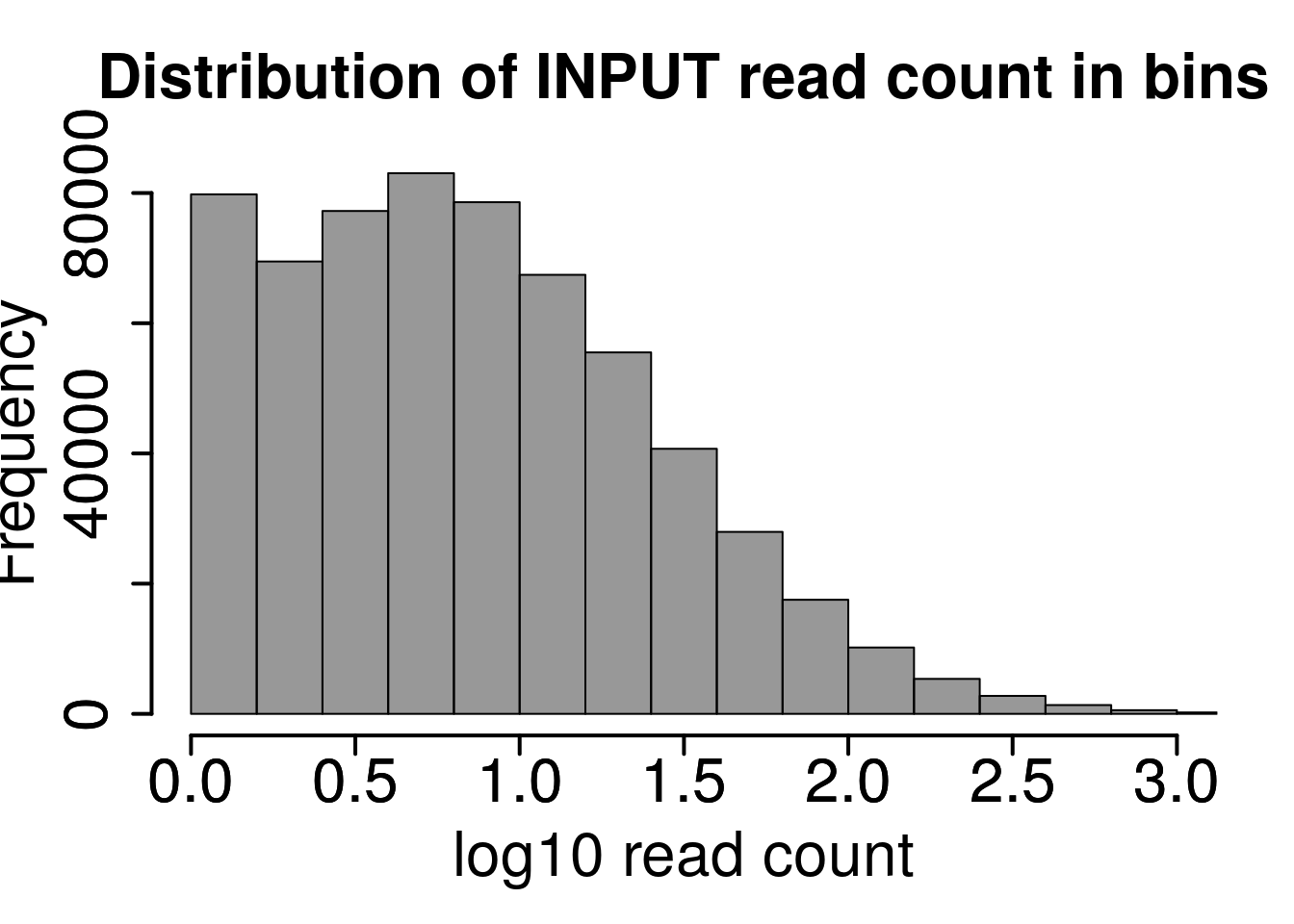
local read count V.S. geneSum
Compute the within group variability of INPUT geneSum VS INPUT local read count.
var.coef <- function(x){sd(as.numeric(x))/mean(as.numeric(x))}
## filter expressed genes
geneSum <- RADAR@geneSum[rowSums(RADAR@geneSum)>16,]
## within group variability
relative.var <- t( apply(geneSum,1,tapply,unlist(variable(RADAR)[,1]),var.coef) )
geneSum.var <- c(relative.var)

## For each gene used above, random sample a 50bp bin within this gene
set.seed(1)
r.bin50 <- tapply(rownames(RADAR@norm.input)[which(RADAR@geneBins$gene %in% rownames(geneSum))],as.character( RADAR@geneBins$gene[which(RADAR@geneBins$gene %in% rownames(geneSum))]) ,function(x){
  n <- sample(1:length(x),1)
  return(x[n])
})

relative.var <- apply(RADAR@norm.input[r.bin50,],1,tapply,unlist(variable(RADAR)[,1]),var.coef)
bin50.var <- c(relative.var)
bin50.var <- bin50.var[!is.na(bin50.var)]

## 100bp bins
r.bin100 <- tapply(rownames(RADAR@norm.input)[which(RADAR@geneBins$gene %in% rownames(geneSum))],as.character( RADAR@geneBins$gene[which(RADAR@geneBins$gene %in% rownames(geneSum))]) ,function(x){
  n <- sample(1:(length(x)-2),1)
  return(x[n:(n+1)])
})
relative.var <- lapply(r.bin100, function(x){ tapply( colSums(RADAR@norm.input[x,]),unlist(variable(RADAR)[,1]),var.coef ) })
bin100.var <- unlist(relative.var)
bin100.var <- bin100.var[!is.na(bin100.var)]

## 200bp bins
r.bin200 <- tapply(rownames(RADAR@norm.input)[which(RADAR@geneBins$gene %in% rownames(geneSum))],as.character( RADAR@geneBins$gene[which(RADAR@geneBins$gene %in% rownames(geneSum))]) ,function(x){
  if(length(x)>4){
    n <- sample(1:(length(x)-3),1)
    return(x[n:(n+3)])
  }else{
    return(NULL)
  }
})
r.bin200 <- r.bin200[which(!unlist(lapply(r.bin200,is.null)) ) ]
relative.var <- lapply(r.bin200, function(x){ tapply( colSums(RADAR@norm.input[x,]),unlist(variable(RADAR)[,1]),var.coef ) })

bin200.var <- unlist(relative.var)
bin200.var <- bin200.var[!is.na(bin200.var)]

relative.var <- data.frame(group=c(rep("geneSum",length(geneSum.var)),rep("bin-50bp",length(bin50.var)),rep("bin-100bp",length(bin100.var)),rep("bin-200bp",length(bin200.var))), variance=c(geneSum.var,bin50.var,bin100.var,bin200.var))ggplot(relative.var,aes(variance,colour=group))+geom_density()+xlab("Relative variation")+
theme_bw() + theme(panel.border = element_blank(), panel.grid.major = element_blank(),
panel.grid.minor = element_blank(), axis.line = element_line(colour = "black",size = 1),
axis.title.x=element_text(size=20, face="bold", hjust=0.5,family = "arial"),
axis.title.y=element_text(size=20, face="bold", vjust=0.4, angle=90,family = "arial"),
legend.position = c(0.88,0.88),legend.title=element_blank(),legend.text = element_text(size = 14, face = "bold",family = "arial"),
axis.text = element_text(size = 15,face = "bold",family = "arial",colour = "black") )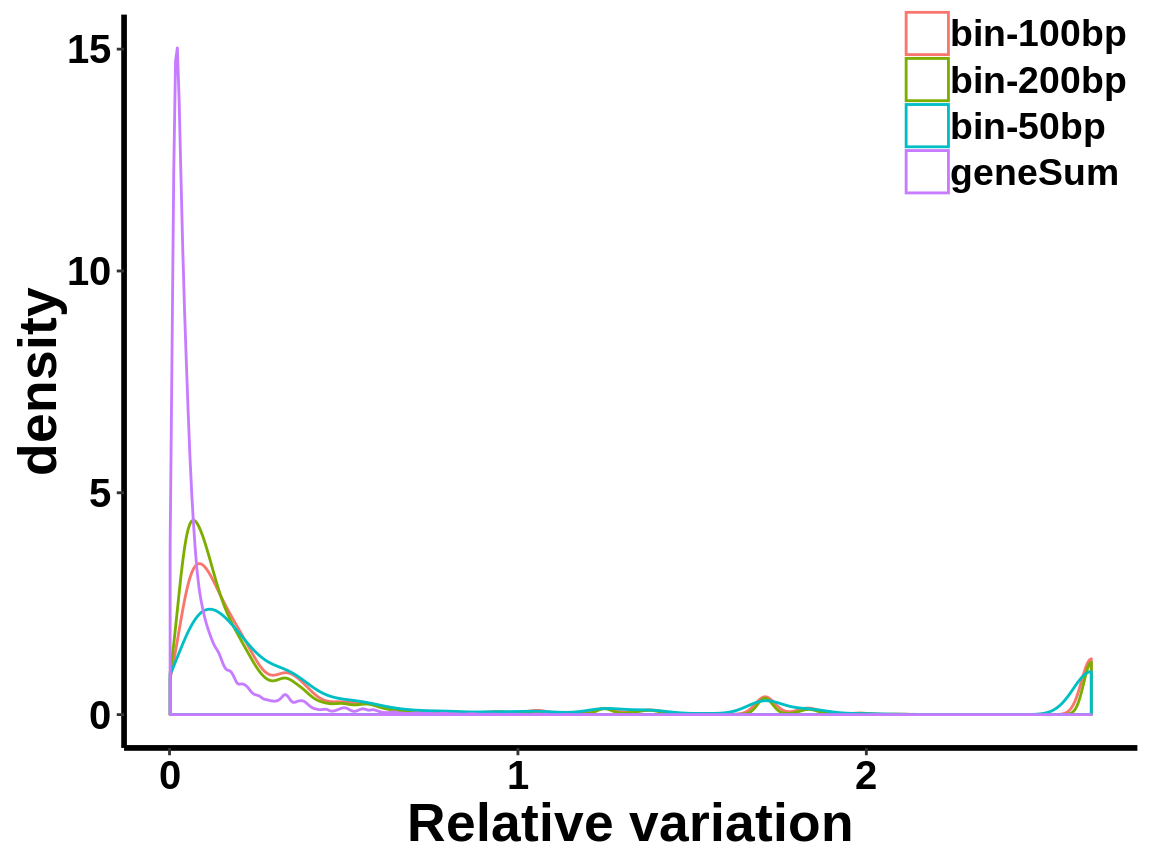
Check mean variance relationship of the data.
ip_var <- t(apply(RADAR@ip_adjExpr_filtered,1,tapply,unlist(variable(RADAR)[,1]),var))
#ip_var <- ip_coef_var[!apply(ip_var,1,function(x){return(any(is.na(x)))}),]
ip_mean <- t(apply(RADAR@ip_adjExpr_filtered,1,tapply,unlist(variable(RADAR)[,1]),mean))

###
gene_var <-  t(apply(RADAR@geneSum,1,tapply,unlist(variable(RADAR)[,1]),var))
#gene_var <- gene_var[!apply(gene_var,1,function(x){return(any(is.na(x)))}),]
gene_mean <- t(apply(RADAR@geneSum,1,tapply,unlist(variable(RADAR)[,1]),mean))

all_var <- list('RNA-seq'=c(gene_var),'m6A-IP'=c(ip_var))
nn<-sapply(all_var, length)
rs<-cumsum(nn)
re<-rs-nn+1
group <- factor(rep(names(all_var), nn), levels=names(all_var))
all_var.df <- data.frame(variance = c(c(gene_var),c(ip_var)),mean= c(c(gene_mean),c(ip_mean)),label = group)ggplot(data = all_var.df,aes(x=mean,y=variance,colour = label,shape = label))+geom_point(size = I(0.2))+stat_smooth(se = T,show.legend = F)+stat_smooth(se = F)+theme_bw() +xlab("Mean")+ ylab("Variance")+theme(panel.border = element_blank(), panel.grid.major = element_blank(),
panel.grid.minor = element_blank(), axis.line = element_line(colour = "black",size = 1),
axis.title.x=element_text(size=22, face="bold", hjust=0.5,family = "arial"),
axis.title.y=element_text(size=22, face="bold", vjust=0.4, angle=90,family = "arial"),
legend.position = c(0.85,0.95),legend.title=element_blank(),legend.text = element_text(size = 20, face = "bold",family = "arial"),
axis.text = element_text(size = 15,face = "bold",family = "arial",colour = "black") ) +
scale_x_continuous(limits = c(0,10000))+scale_y_continuous(limits = c(0,6e5))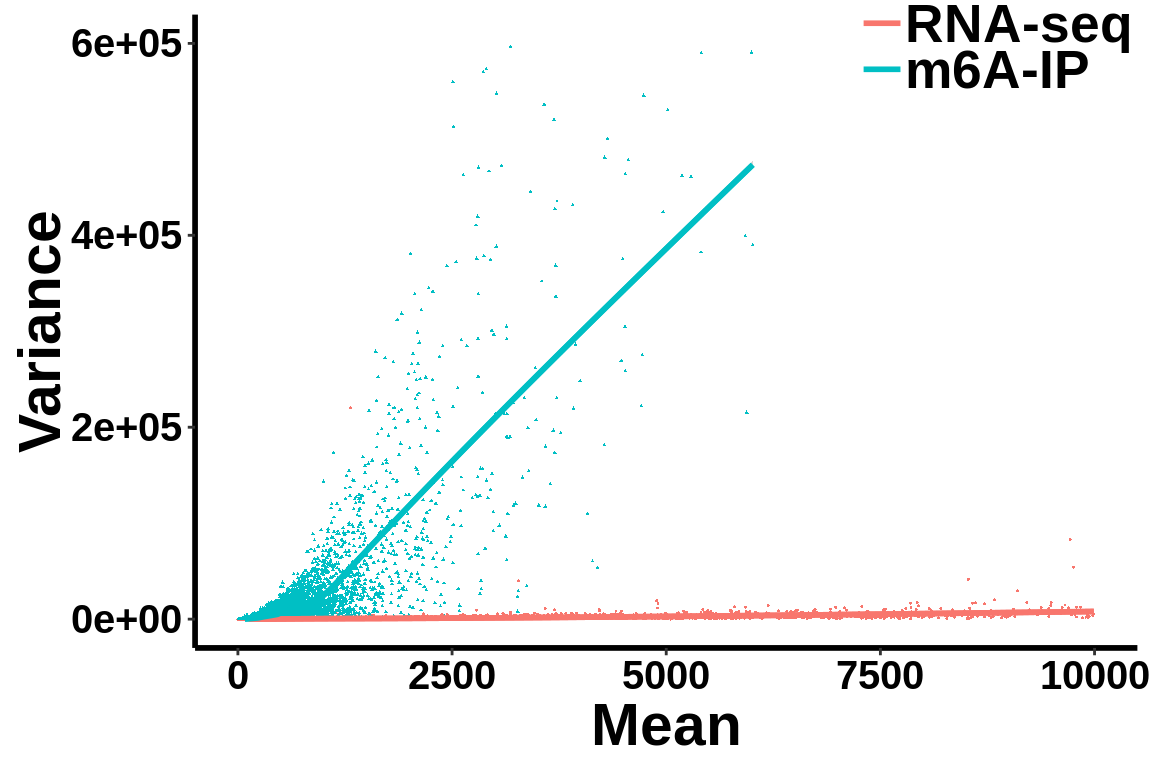
ggplot(data = all_var.df,aes(x=mean,y=variance,colour = label,shape = label))+geom_point(size = I(0.2))+stat_smooth(data = all_var.df[all_var.df$label=="RNA-seq",],se = T,show.legend = F )+stat_smooth(data = all_var.df[all_var.df$label=="RNA-seq",],se = F)+theme_bw() +xlab("Mean")+ ylab("Variance")+theme(panel.border = element_blank(), panel.grid.major = element_blank(),
                   panel.grid.minor = element_blank(), axis.line = element_line(colour = "black",size = 1),
                   axis.title.x=element_text(size=22, face="bold", hjust=0.5,family = "arial"),
                   axis.title.y=element_text(size=22, face="bold", vjust=0.4, angle=90,family = "arial"),
                   legend.position = c(0.85,0.95),legend.title=element_blank(),legend.text = element_text(size = 20, face = "bold",family = "arial"),
                   axis.text = element_text(size = 15,face = "bold",family = "arial",colour = "black") ) +
  scale_x_continuous(limits = c(0,10000))+scale_y_continuous(limits = c(0,2e4))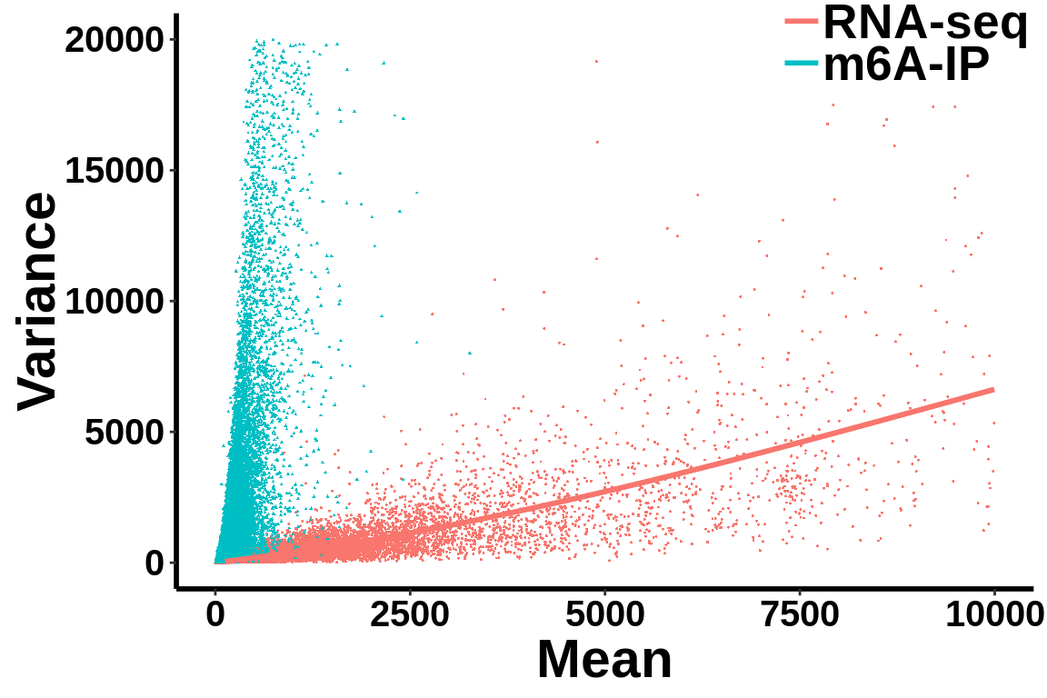
Compare MeRIP-seq IP data with regular RNA-seq data
var.coef <- function(x){sd(as.numeric(x))/mean(as.numeric(x))}

ip_coef_var <- t(apply(RADAR@ip_adjExpr_filtered,1,tapply,unlist(variable(RADAR)[,1]),var.coef))
ip_coef_var <- ip_coef_var[!apply(ip_coef_var,1,function(x){return(any(is.na(x)))}),]
#hist(c(ip_coef_var),main = "M14KO mouse liver\n m6A-IP",xlab = "within group coefficient of variation",breaks = 50)
###
gene_coef_var <-  t(apply(RADAR@geneSum,1,tapply,unlist(variable(RADAR)[,1]),var.coef))
gene_coef_var <- gene_coef_var[!apply(gene_coef_var,1,function(x){return(any(is.na(x)))}),]
#hist(c(gene_coef_var),main = "M14KO mouse liver\n RNA-seq",xlab = "within group coefficient of variation",breaks = 50)

coef_var <- list('RNA-seq'=c(gene_coef_var),'m6A-IP'=c(ip_coef_var))
nn<-sapply(coef_var, length)
rs<-cumsum(nn)
re<-rs-nn+1
grp <- factor(rep(names(coef_var), nn), levels=names(coef_var))
coef_var.df <- data.frame(coefficient_var = c(c(gene_coef_var),c(ip_coef_var)),label = grp)ggplot(data = coef_var.df,aes(coefficient_var,colour = grp))+geom_density()+theme_bw() +theme(panel.border = element_blank(), panel.grid.major = element_blank(),
panel.grid.minor = element_blank(), axis.line = element_line(colour = "black",size = 1),
axis.title.x=element_text(size=20, face="bold", hjust=0.5,family = "arial"),
axis.title.y=element_text(size=20, face="bold", vjust=0.4, angle=90,family = "arial"),
legend.position = c(0.9,0.9),legend.title=element_blank(),legend.text = element_text(size = 18, face = "bold",family = "arial"),
axis.text = element_text(size = 15,face = "bold",family = "arial",colour = "black") )+
xlab("Coefficient of variation")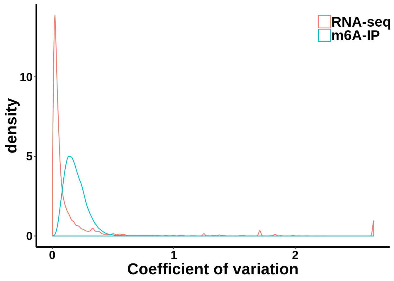
Plot PCA
We plot PCA colored by Ctl vs Tumor
plotPCAfromMatrix(RADAR@ip_adjExpr_filtered,group = unlist(variable(RADAR)[,1]) )+scale_color_discrete(name = "Group")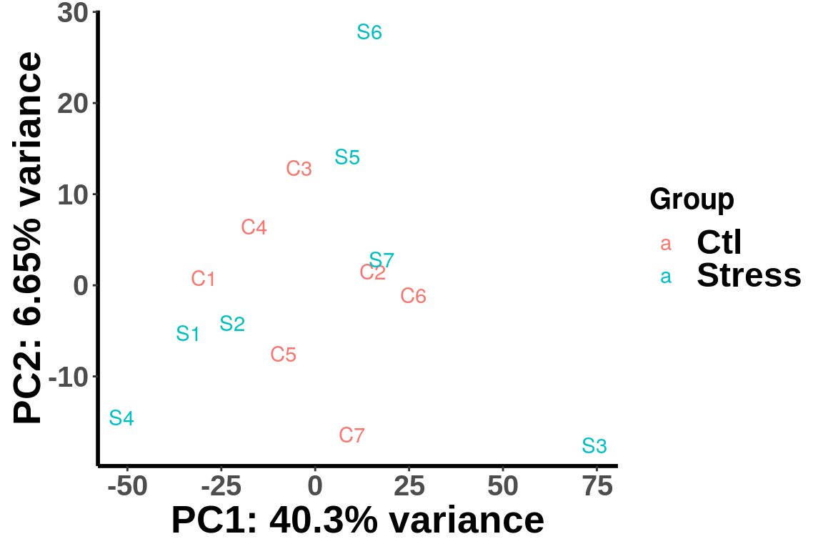
(Adjust expression level by local read count)
plotPCAfromMatrix(RADAR_pos@ip_adjExpr_filtered,group = unlist(variable(RADAR)[,1]) )+scale_color_discrete(name = "Group")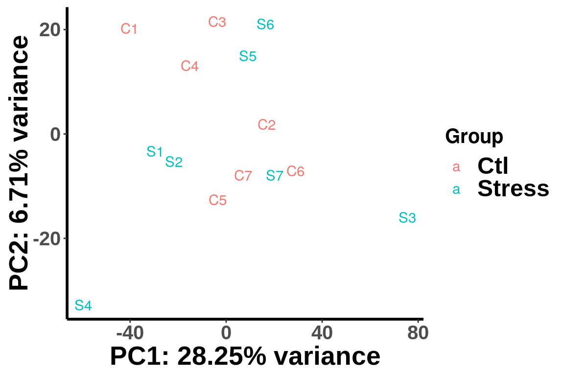
Compare methods
PoissonGamma Test
RADAR <-  diffIP_parallel(RADAR,thread = 25  , fdrBy = "fdr")
RADAR_pos <-  diffIP_parallel(RADAR_pos,thread = 25 ,fdrBy = "fdr")
Other method
## fisher's exact test
fisherTest <- function( control_ip, treated_ip, control_input, treated_input, thread ){
  registerDoParallel(cores = thread)
  testResult <- foreach(i = 1:nrow(control_ip) , .combine = rbind )%dopar%{
    tmpTest <- fisher.test( cbind( c( rowSums(treated_ip)[i], rowSums(treated_input)[i] ), c( rowSums(control_ip)[i], rowSums(control_input)[i] ) ), alternative = "two.sided" )
    data.frame( logFC = log(tmpTest$estimate), pvalue =  tmpTest$p.value )
  }
  rm(list=ls(name=foreach:::.foreachGlobals), pos=foreach:::.foreachGlobals)
  testResult$fdr <- p.adjust(testResult$pvalue, method = "fdr")
  return(testResult)
}

## wrapper for the MetDiff test
MeTDiffTest <-  function( control_ip, treated_ip, control_input, treated_input, thread = 1 ){
  registerDoParallel(cores = thread)
  testResult <- foreach(i = 1:nrow(control_ip) , .combine = rbind )%dopar%{
    x <- t( as.matrix(control_ip[i,]) )
    y <- t( as.matrix(control_input[i,]) )
    xx <- t( as.matrix(treated_ip[i,]) )
    yy <- t( as.matrix(treated_input[i,]) )
    xxx = cbind(x,xx)
    yyy = cbind(y,yy)

    logl1 <- MeTDiff:::.betabinomial.lh(x,y+1)
    logl2 <- MeTDiff:::.betabinomial.lh(xx,yy+1)
    logl3 <- MeTDiff:::.betabinomial.lh(xxx,yyy+1)
    tst <- (logl1$logl+logl2$logl-logl3$logl)*2
    pvalues <- 1 - pchisq(tst,2)
    log.fc <- log( (sum(xx)+1)/(1+sum(yy)) * (1+sum(y))/(1+sum(x)) )

    data.frame( logFC = log.fc, pvalue =  pvalues )
  }
  rm(list=ls(name=foreach:::.foreachGlobals), pos=foreach:::.foreachGlobals)
  testResult$fdr <- p.adjust(testResult$pvalue, method = "fdr")
  return(testResult)
}


Bltest <- function(control_ip, treated_ip, control_input, treated_input){
  control_ip_total <- sum(colSums(control_ip))
  control_input_total <- sum(colSums(control_input))
  treated_ip_total <- sum(colSums(treated_ip))
  treated_input_total <- sum(colSums(treated_input))

  tmpResult <- do.call(cbind.data.frame, exomePeak::bltest(rowSums(control_ip), rowSums(control_input),rowSums(treated_ip),rowSums(treated_input),control_ip_total, control_input_total, treated_ip_total,  treated_input_total) )
  return( data.frame(logFC = tmpResult[,"log.fc"], pvalue = exp(tmpResult[,"log.p"]), fdr = exp(tmpResult$log.fdr) ) )
}
In order to compare performance of other method on this data set, we run other methods on default mode on this dataset.
filteredBins <- rownames(RADAR@ip_adjExpr_filtered)

 Metdiff.res <-MeTDiffTest(control_ip = round( RADAR@norm.ip[filteredBins,1:7] ) ,
                        treated_ip = round( RADAR@norm.ip[filteredBins,8:14] ),
                        control_input = round( RADAR@norm.input[filteredBins,1:7] ),
                        treated_input = round( RADAR@norm.input[filteredBins,8:14] ) , thread = 20)


  QNB.res <- QNB::qnbtest(control_ip = round( RADAR@norm.ip[filteredBins,1:7] ) ,
                        treated_ip = round( RADAR@norm.ip[filteredBins,8:14] ),
                        control_input = round( RADAR@norm.input[filteredBins,1:7] ),
                        treated_input = round( RADAR@norm.input[filteredBins,8:14] ) ,plot.dispersion = FALSE )

  fisher.res <- fisherTest(control_ip = round( RADAR@norm.ip[filteredBins,1:7] ) ,
                        treated_ip = round( RADAR@norm.ip[filteredBins,8:14] ),
                        control_input = round( RADAR@norm.input[filteredBins,1:7] ),
                        treated_input = round( RADAR@norm.input[filteredBins,8:14] ) )

  exomePeak.res <- Bltest(control_ip = round( RADAR@norm.ip[filteredBins,1:7] ) ,
                        treated_ip = round( RADAR@norm.ip[filteredBins,8:14] ),
                        control_input = round( RADAR@norm.input[filteredBins,1:7] ),
                        treated_input = round( RADAR@norm.input[filteredBins,8:14] ) )
Compare distribution of p value.
pvalues <- data.frame(pvalue = c(RADAR@test.est[,"p_value"],Metdiff.res$pvalue,QNB.res$pvalue,fisher.res$pvalue, exomePeak.res$pvalue ),
                      method = factor(rep(c("RADAR","MeTDiff","QNB","Fisher","exomePeak"),c(length(RADAR@test.est[,"p_value"]),
                                                                       length(Metdiff.res$pvalue),
                                                                       length(QNB.res$pvalue),
                                                                       length(fisher.res$pvalue),
                                                                       length(exomePeak.res$pvalue)
                                                                       )
                                          ),levels =c("RADAR","MeTDiff","QNB","Fisher","exomePeak")
                                   )
                      )
ggplot(pvalues, aes(x = pvalue))+geom_histogram(breaks = seq(0,1,0.04),col=I("black"))+facet_grid(.~method)+theme_bw()+xlab("p-value")+theme( axis.title =  element_text(size = 22, face = "bold"),strip.text = element_text(size = 25, face = "bold"),axis.text.x = element_text(size = 18, face = "bold",colour = "black"),axis.text.y = element_text(size = 15, face = "bold",colour = "black",angle = 90),panel.grid = element_blank(), axis.line = element_line(size = 0.7 ,colour = "black"),axis.ticks = element_line(colour = "black"), panel.spacing = unit(0.4, "lines") )+ scale_x_continuous(breaks = seq(0,1,0.2),labels=function(x) sprintf("%.1f", x))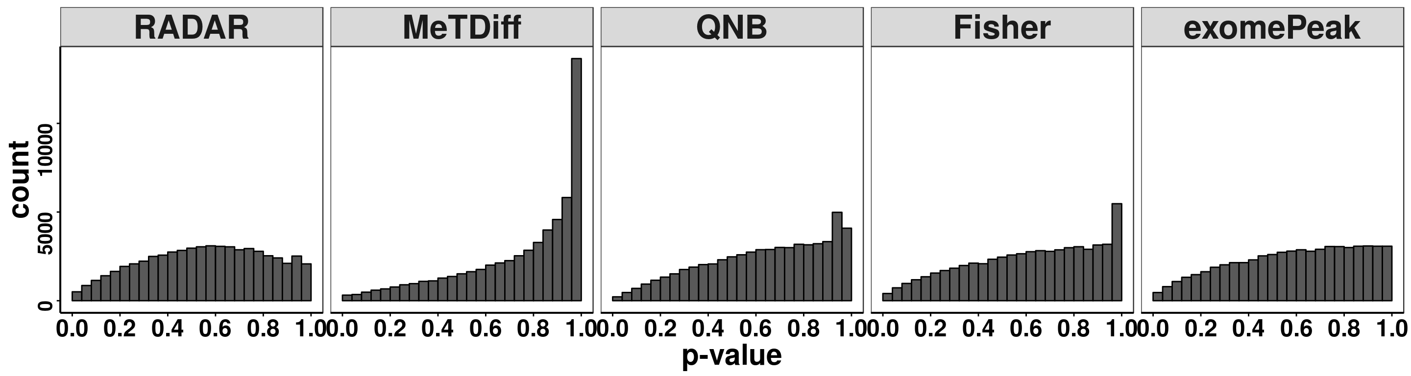
Compare adjusting expression level by geneSum vs. bin read counts.
tmp <- hist(c(RADAR_pos@test.est[,"p_value"]),plot = F)
tmp$counts <- tmp$counts*(nrow(RADAR@ip_adjExpr_filtered)/nrow(RADAR_pos@ip_adjExpr_filtered))
hist(RADAR@test.est[,"p_value"],main = "RADAR",xlab = "p value",col =rgb(1,0,0,0.4),cex.main = 2.5,cex.axis =2,cex.lab=2, ylim = c(0,max(hist(RADAR@test.est[,"p_value"],plot = F)$counts,tmp$counts)+800) )
plot(tmp,col=rgb(0,0,1,0.5),add = T)
axis(side = 1, lwd = 1,cex.axis =2)
axis(side = 2, lwd = 1,cex.axis =2)
legend("topright", c("By geneSum", "By position"), col=c(rgb(1,0,0,0.4), rgb(0,0,1,0.5)), lwd = 10,bty="n",text.font = 2)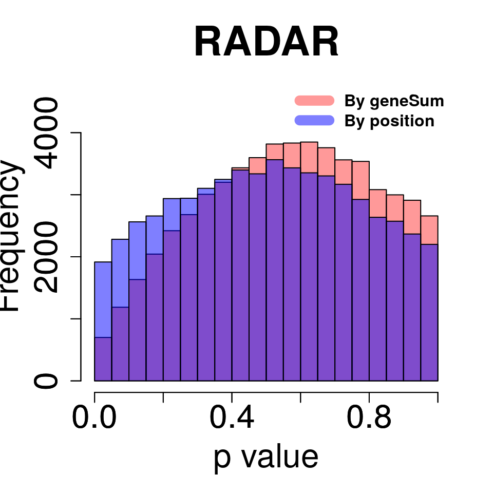
Compare the distibution of beta
par(mfrow = c(1,5))
hist(RADAR@test.est[,"beta"],main = "RADAR",xlab = "beta",breaks = 100,col =rgb(0.2,0.2,0.2,0.5),cex.main = 2.5,cex.axis =2,cex.lab=2)
#hist(radar_byPos$all.est[,"beta1"],main = "Norm by pos",xlab = "beta",breaks = 100)
hist(Metdiff.res$logFC, main = "MeTDiff",xlab = "beta",breaks = 100,col =rgb(0.2,0.2,0.2,0.5),cex.main = 2.5,cex.axis =2,cex.lab=2)
hist(QNB.res$log2.OR,main = "QNB", xlab = "beta",breaks = 100,col =rgb(0.2,0.2,0.2,0.5),cex.main = 2.5,cex.axis =2,cex.lab=2)
hist(fisher.res$logFC, main = "Fisher",xlab = "beta",breaks = 100,col =rgb(0.2,0.2,0.2,0.5),cex.main = 2.5,cex.axis =2,cex.lab=2)
hist(exomePeak.res$logFC, main = "exomePeak",xlab = "beta",breaks = 100,col =rgb(0.2,0.2,0.2,0.5),cex.main = 2.5,cex.axis =2,cex.lab=2)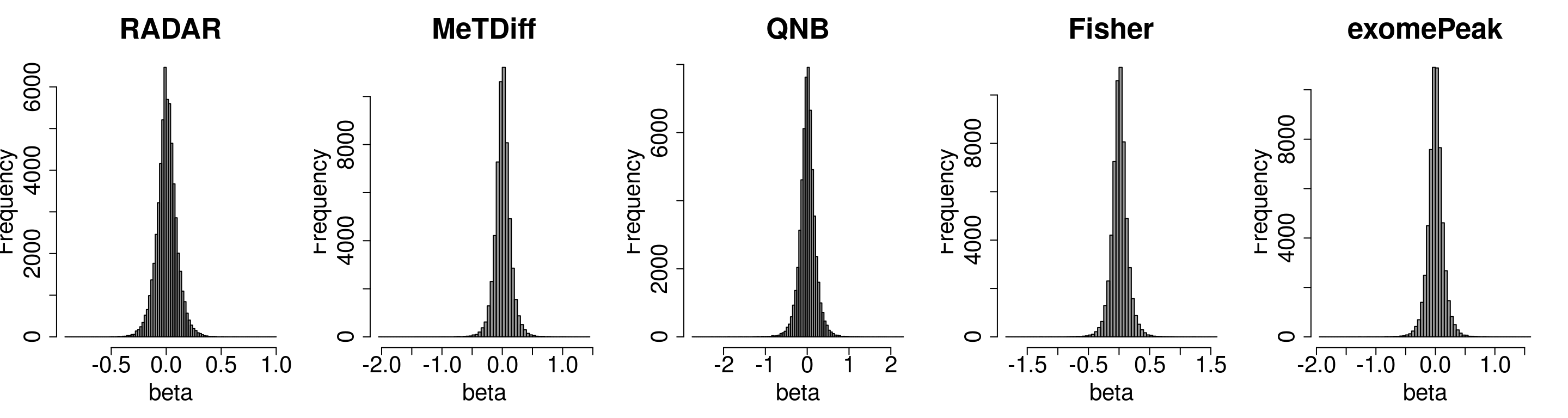
Number of significant bins detected at FDR < 0.1.
sigBins <- apply(cbind("RADAR"=RADAR@test.est[,"p_value"],"MeTDiff"=Metdiff.res$pvalue,"QNB"=QNB.res$pvalue,"Fisher"=fisher.res$pvalue,"exomePeak" = exomePeak.res$pvalue),2, function(x){
  length( which( p.adjust(x,method = 'fdr') < 0.1 ) )
})
print(sigBins)
## RADAR MeTDiff QNB Fisher exomePeak
## 0 105 2 3 3Permutation Test
radar_permuted_P <-NULL
metdiff_permuted_P <- NULL
qnb_permuted_P <- NULL
fisher_permuted_P <- NULL
exomePeak_permute_P <- NULL

set.seed(2)
for(i in 1:15){

  permute_X <- variable(RADAR)[,1]
  permute_X[sample(1:7, sample(3:4,1) )] <- "Stress"
  permute_X[sample(8:14, sample(3:4,1) )] <- "Ctl"
  RADAR_permute <- RADAR
  variable(RADAR_permute) <- data.frame(condition = permute_X  )

  radar_permute <- diffIP_parallel( RADAR_permute , thread = 20 )@test.est[,"p_value"]

  metdiff_permute <-MeTDiffTest( control_ip = round( RADAR@norm.ip[filteredBins ,(which(permute_X == "Ctl" ) )] ),
                                 treated_ip = round( RADAR@norm.ip[filteredBins,(which(permute_X == "Stress" ) )] ),
                                 control_input = round( RADAR@norm.input[filteredBins,which(permute_X == "Ctl" )] ),
                                 treated_input = round( RADAR@norm.input[filteredBins,which(permute_X == "Stress" )] ) ,
                                 thread = 25)$pvalue

  qnb_permute <- QNB::qnbtest(control_ip = round( RADAR@norm.ip[filteredBins ,(which(permute_X == "Ctl" ) )] ),
                              treated_ip = round( RADAR@norm.ip[filteredBins,(which(permute_X == "Stress" ) )] ),
                              control_input = round( RADAR@norm.input[filteredBins,which(permute_X == "Ctl" )] ),
                              treated_input = round( RADAR@norm.input[filteredBins,which(permute_X == "Stress" )] ),
                              plot.dispersion = FALSE)$pvalue

  fisher_permute <- fisherTest( control_ip = round( RADAR@norm.ip[filteredBins ,(which(permute_X == "Ctl" ) )] ),
                                treated_ip = round( RADAR@norm.ip[filteredBins,(which(permute_X == "Stress" ) )] ),
                                control_input = round( RADAR@norm.input[filteredBins,which(permute_X == "Ctl" )] ),
                                treated_input = round( RADAR@norm.input[filteredBins,which(permute_X == "Stress" )] )  ,
                                thread = 25
                               )$pvalue

  exomePeak_permute <- Bltest( control_ip = round( RADAR@norm.ip[filteredBins ,(which(permute_X == "Ctl" ) )] ),
                               treated_ip = round( RADAR@norm.ip[filteredBins,(which(permute_X == "Stress" ) )] ),
                               control_input = round( RADAR@norm.input[filteredBins,which(permute_X == "Ctl" )] ),
                               treated_input = round( RADAR@norm.input[filteredBins,which(permute_X == "Stress" )] )
                              )$pvalue

  radar_permuted_P <- cbind(radar_permuted_P, radar_permute)
  metdiff_permuted_P <- cbind(metdiff_permuted_P, metdiff_permute)
  qnb_permuted_P <- cbind(qnb_permuted_P,qnb_permute)
  fisher_permuted_P <- cbind(fisher_permuted_P, fisher_permute)
  exomePeak_permute_P <- cbind(exomePeak_permute_P, exomePeak_permute)

}

for( i in 1:ncol(radar_permuted_P)){
par(mfrow=c(1,5))
hist(RADAR@test.est[,"p_value"], col =rgb(1,0,0,0.4),main = "RADAR", xlab = "p value",cex.main = 2.5,cex.axis =2,cex.lab=2)
hist(radar_permuted_P[,i],col=rgb(0,0,1,0.5),add = T)
legend("topright", c("Original", "Permuted"), col=c(rgb(1,0,0,0.4), rgb(0,0,1,0.5)), lwd = 10,bty="n")
hist(Metdiff.res$pvalue, col =rgb(1,0,0,0.4),main = "MeTdiff",xlab = "p value",cex.main = 2.5,cex.axis =2,cex.lab=2)
hist(metdiff_permuted_P[,i],col=rgb(0,0,1,0.5),add = T)
legend("topright", c("Original", "Permuted"), col=c(rgb(1,0,0,0.4), rgb(0,0,1,0.5)), lwd = 10,bty="n")
hist(QNB.res$pvalue, col =rgb(1,0,0,0.4),main = "QNB",xlab = "p value",cex.main = 2.5,cex.axis =2,cex.lab=2)
hist(qnb_permuted_P[,i],col=rgb(0,0,1,0.5),add = T)
legend("topright", c("Original", "Permuted"), col=c(rgb(1,0,0,0.4), rgb(0,0,1,0.5)), lwd = 10,bty="n")
hist(fisher.res$pvalue, col =rgb(1,0,0,0.4),main = "Fisher",xlab = "p value",cex.main = 2.5,cex.axis =2,cex.lab=2)
hist(fisher_permuted_P[,i],col=rgb(0,0,1,0.5),add = T)
legend("topright", c("Original", "Permuted"), col=c(rgb(1,0,0,0.4), rgb(0,0,1,0.5)), lwd = 10,bty="n")
hist(exomePeak.res$pvalue, col =rgb(1,0,0,0.4),main = "exomePeak",xlab = "p value",cex.main = 2.5,cex.axis =2,cex.lab=2)
hist(exomePeak_permute_P[,i],col=rgb(0,0,1,0.5),add = T)
legend("topright", c("Original", "Permuted"), col=c(rgb(1,0,0,0.4), rgb(0,0,1,0.5)), lwd = 10,bty="n")

}par(mfrow=c(1,5))
y.scale <- max(hist(Metdiff.res$pvalue,plot = F)$counts)+3000
hist(RADAR@test.est[,"p_value"], col =rgb(1,0,0,0.4),main = "RADAR", xlab = "p value",font=2, cex.lab=2.5, cex.axis = 1.5 , font.lab=2 ,cex.main = 3, lwd = 3, ylim = c(0,y.scale) )
tmp <- hist(c(radar_permuted_P),plot = F)
tmp$counts <- tmp$counts/15
plot(tmp,col=rgb(0,0,1,0.5),add = T)
legend("topright", c("Original", "Permuted"), col=c(rgb(1,0,0,0.4), rgb(0,0,1,0.5)), lwd = 12,bty="n",text.font = 2, cex = 1.5)
tmp <- hist(c(metdiff_permuted_P),plot = F)
tmp$counts <- tmp$counts/15
hist(Metdiff.res$pvalue, col =rgb(1,0,0,0.4),main = "MeTDiff",xlab = "p value" ,font=2, cex.lab=2.5, cex.axis = 1.5 , font.lab=2 ,cex.main = 3, lwd = 3, ylim = c(0,y.scale) )
plot(tmp,col=rgb(0,0,1,0.5),add = T)
legend("topright", c("Original", "Permuted"), col=c(rgb(1,0,0,0.4), rgb(0,0,1,0.5)), lwd = 12,bty="n",text.font = 2, cex = 1.5)
hist(QNB.res$pvalue, col =rgb(1,0,0,0.4),main = "QNB",xlab = "p value",font=2, cex.lab=2.5, cex.axis = 1.5 , font.lab=2 ,cex.main = 3,lwd = 3,ylim = c(0,y.scale))
tmp <- hist(c(qnb_permuted_P),plot = F)
tmp$counts <- tmp$counts/15
plot(tmp,col=rgb(0,0,1,0.5),add = T)
legend("topright", c("Original", "Permuted"), col=c(rgb(1,0,0,0.4), rgb(0,0,1,0.5)), lwd = 12,bty="n",text.font = 2, cex = 1.5)
hist(fisher.res$pvalue, col =rgb(1,0,0,0.4),main = "Fisher",xlab = "p value",font=2, cex.lab=2.5, cex.axis = 1.5 , font.lab=2 ,cex.main = 3,lwd = 3,ylim = c(0,y.scale))
tmp <- hist(c(fisher_permuted_P),plot = F)
tmp$counts <- tmp$counts/15
plot(tmp,col=rgb(0,0,1,0.5),add = T)
legend("topright", c("Original", "Permuted"), col=c(rgb(1,0,0,0.4), rgb(0,0,1,0.5)), lwd = 12,bty="n",text.font = 2, cex = 1.5)
hist(exomePeak.res$pvalue, col =rgb(1,0,0,0.4),main = "exomePeak",xlab = "p value",font=2, cex.lab=2.5, cex.axis = 1.5 , font.lab=2 ,cex.main = 3,lwd = 3,ylim = c(0,y.scale))
tmp <- hist(c(exomePeak_permute_P),plot = F)
tmp$counts <- tmp$counts/15
plot(tmp,col=rgb(0,0,1,0.5),add = T)
legend("topright", c("Original", "Permuted"), col=c(rgb(1,0,0,0.4), rgb(0,0,1,0.5)), lwd = 12,bty="n",text.font = 2, cex = 1.5)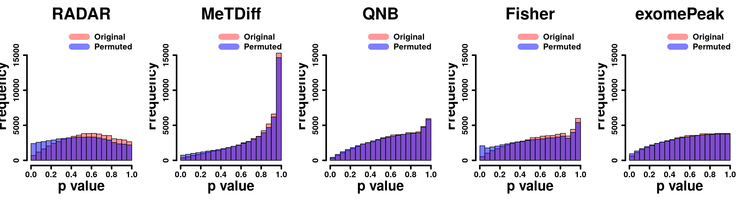
Permutation by position
radar_permuted_P_pos <-NULL

set.seed(2)
for(i in 1:15){

  permute_X <- variable(RADAR)[,1]
  permute_X[sample(1:7, sample(3:4,1) )] <- "Stress"
  permute_X[sample(8:14, sample(3:4,1) )] <- "Ctl"
  RADAR_permute <- RADAR_pos
  variable(RADAR_permute) <- data.frame(condition = permute_X  )

  radar_permute <- diffIP_parallel( RADAR_permute , thread = 20 )@test.est[,"p_value"]

  radar_permuted_P_pos <- cbind(radar_permuted_P_pos, radar_permute)

} par(mfrow=c(1,2))
y.scale <- max(hist( RADAR@test.est[,"p_value"] ,plot = F)$counts)+1000
hist(RADAR@test.est[,"p_value"], col =rgb(1,0,0,0.4),main = "RADAR by geneSum", xlab = "p value",font=2, cex.lab=2.5, cex.axis = 1.5 , font.lab=2 ,cex.main = 3, lwd = 3, ylim = c(0,y.scale) )
tmp <- hist(c(radar_permuted_P),plot = F)
tmp$counts <- tmp$counts/15
plot(tmp,col=rgb(0,0,1,0.5),add = T)
legend("topright", c("Original", "Permuted"), col=c(rgb(1,0,0,0.4), rgb(0,0,1,0.5)), lwd = 12,bty="n",text.font = 2, cex = 1.5)
hist(RADAR_pos@test.est[,"p_value"], col =rgb(1,0,0,0.4),main = "RADAR by pos", xlab = "p value",font=2, cex.lab=2.5, cex.axis = 1.5 , font.lab=2 ,cex.main = 3, lwd = 3, ylim = c(0,y.scale) )
tmp <- hist(c(radar_permuted_P_pos),plot = F)
tmp$counts <- tmp$counts/15
plot(tmp,col=rgb(0,0,1,0.5),add = T)
legend("topright", c("Original", "Permuted"), col=c(rgb(1,0,0,0.4), rgb(0,0,1,0.5)), lwd = 12,bty="n",text.font = 2, cex = 1.5)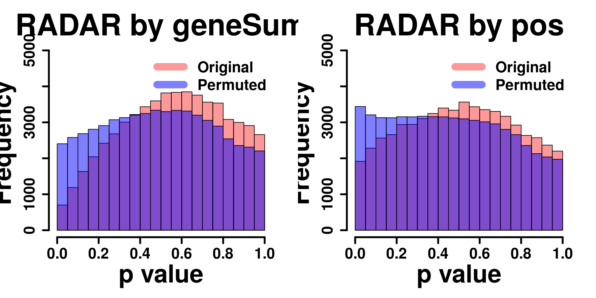
Session information
sessionInfo()## R version 3.5.3 (2019-03-11)
## Platform: x86_64-pc-linux-gnu (64-bit)
## Running under: Ubuntu 17.10
##
## Matrix products: default
## BLAS: /usr/lib/x86_64-linux-gnu/openblas/libblas.so.3
## LAPACK: /usr/lib/x86_64-linux-gnu/libopenblasp-r0.2.20.so
##
## locale:
## [1] LC_CTYPE=en_US.UTF-8 LC_NUMERIC=C
## [3] LC_TIME=en_US.UTF-8 LC_COLLATE=en_US.UTF-8
## [5] LC_MONETARY=en_US.UTF-8 LC_MESSAGES=en_US.UTF-8
## [7] LC_PAPER=en_US.UTF-8 LC_NAME=C
## [9] LC_ADDRESS=C LC_TELEPHONE=C
## [11] LC_MEASUREMENT=en_US.UTF-8 LC_IDENTIFICATION=C
##
## attached base packages:
## [1] stats4 parallel stats graphics grDevices utils datasets
## [8] methods base
##
## other attached packages:
## [1] RADAR_0.2.0 qvalue_2.14.1
## [3] RcppArmadillo_0.9.400.2.0 Rcpp_1.0.1
## [5] RColorBrewer_1.1-2 gplots_3.0.1.1
## [7] doParallel_1.0.14 iterators_1.0.10
## [9] foreach_1.4.4 ggplot2_3.1.1
## [11] Rsamtools_1.34.1 Biostrings_2.50.2
## [13] XVector_0.22.0 GenomicFeatures_1.34.8
## [15] AnnotationDbi_1.44.0 Biobase_2.42.0
## [17] GenomicRanges_1.34.0 GenomeInfoDb_1.18.2
## [19] IRanges_2.16.0 S4Vectors_0.20.1
## [21] BiocGenerics_0.28.0
##
## loaded via a namespace (and not attached):
## [1] backports_1.1.4 Hmisc_4.2-0
## [3] fastmatch_1.1-0 plyr_1.8.4
## [5] igraph_1.2.4.1 lazyeval_0.2.2
## [7] splines_3.5.3 BiocParallel_1.16.6
## [9] urltools_1.7.3 digest_0.6.18
## [11] htmltools_0.3.6 GOSemSim_2.8.0
## [13] viridis_0.5.1 GO.db_3.7.0
## [15] gdata_2.18.0 magrittr_1.5
## [17] checkmate_1.9.1 memoise_1.1.0
## [19] cluster_2.0.7-1 annotate_1.60.1
## [21] matrixStats_0.54.0 enrichplot_1.2.0
## [23] prettyunits_1.0.2 colorspace_1.4-1
## [25] blob_1.1.1 ggrepel_0.8.0
## [27] xfun_0.6 dplyr_0.8.0.1
## [29] crayon_1.3.4 RCurl_1.95-4.12
## [31] jsonlite_1.6 genefilter_1.64.0
## [33] survival_2.44-1.1 glue_1.3.1
## [35] polyclip_1.10-0 gtable_0.3.0
## [37] zlibbioc_1.28.0 UpSetR_1.3.3
## [39] DelayedArray_0.8.0 scales_1.0.0
## [41] DOSE_3.8.2 DBI_1.0.0
## [43] viridisLite_0.3.0 xtable_1.8-4
## [45] progress_1.2.0 htmlTable_1.13.1
## [47] gridGraphics_0.3-0 foreign_0.8-71
## [49] bit_1.1-14 europepmc_0.3
## [51] Formula_1.2-3 htmlwidgets_1.3
## [53] httr_1.4.0 fgsea_1.8.0
## [55] acepack_1.4.1 pkgconfig_2.0.2
## [57] XML_3.98-1.19 farver_1.1.0
## [59] nnet_7.3-12 locfit_1.5-9.1
## [61] ggplotify_0.0.3 tidyselect_0.2.5
## [63] labeling_0.3 rlang_0.3.4
## [65] reshape2_1.4.3 munsell_0.5.0
## [67] tools_3.5.3 RSQLite_2.1.1
## [69] ggridges_0.5.1 evaluate_0.13
## [71] stringr_1.4.0 yaml_2.2.0
## [73] knitr_1.22 bit64_0.9-7
## [75] fs_1.3.0 caTools_1.17.1.2
## [77] purrr_0.3.2 ggraph_1.0.2
## [79] nlme_3.1-137 DO.db_2.9
## [81] xml2_1.2.0 biomaRt_2.38.0
## [83] compiler_3.5.3 rstudioapi_0.10
## [85] tibble_2.1.1 tweenr_1.0.1
## [87] geneplotter_1.60.0 stringi_1.4.3
## [89] lattice_0.20-38 Matrix_1.2-17
## [91] pillar_1.3.1 triebeard_0.3.0
## [93] data.table_1.12.2 cowplot_0.9.4
## [95] bitops_1.0-6 rtracklayer_1.42.2
## [97] R6_2.4.0 latticeExtra_0.6-28
## [99] KernSmooth_2.23-15 gridExtra_2.3
## [101] codetools_0.2-16 MASS_7.3-51.4
## [103] gtools_3.8.1 assertthat_0.2.1
## [105] SummarizedExperiment_1.12.0 DESeq2_1.22.2
## [107] withr_2.1.2 GenomicAlignments_1.18.1
## [109] GenomeInfoDbData_1.2.0 mgcv_1.8-28
## [111] hms_0.4.2 clusterProfiler_3.10.1
## [113] grid_3.5.3 rpart_4.1-13
## [115] tidyr_0.8.3 rmarkdown_1.12
## [117] rvcheck_0.1.3 ggforce_0.2.2
## [119] base64enc_0.1-3This R Markdown site was created with workflowr