MouseLiver

Count reads

library(RADAR)

samplenames = c("4582WT","4584WT","4587WT","4612WT","4583KO","4586KO","4615KO","4616KO")

RADAR <- countReads(samplenames = samplenames,
                  gtf = "/home/zijiezhang/Database/genome/mm10/mm10_UCSC.gtf",
                  bamFolder = "~/METTL14_liver2017/bam_files/",
                  outputDir = "~/METTL14/RADAR",
                  modification = "m6A",
                  threads = 8
)

Summary of read count

library(RADAR)
#load("~/METTL14_liver2017/RDM.RData")
load("~/Tools/RADARmannual/data/mouse_liver_RADAR_analysis.RData")
summary(RADAR)

## MeRIP.RADAR dataset of 8 samples.
## Read count quantified in 50-bp consecutive bins on the transcript.
## The total read count for Input and IP samples are (Million reads):
##       4582WT 4584WT 4587WT 4612WT 4583KO 4586KO 4615KO 4616KO
## Input  19.23  16.78  16.61  17.36  22.42  17.88  17.24  18.96
## IP     18.79  21.71  19.98  20.28  19.22  21.70  20.87  18.26
## Input gene level read count available.
## There are 1 predictor variables/covariates. Can access by function variable(MeRIPdata). 
## Differential methylation tested by PoissonGamma test (RADAR).
## Multiple test corrected by Benjamini & Hochberg.
## Neighboring significant bins merged. There are 632 reported differential loci at FDR < 0.1 and logFoldChange > 0.5.

RADAR <- normalizeLibrary(RADAR)
RADAR <- adjustExprLevel(RADAR)

variable(RADAR) <- data.frame( condition = c(rep("WT",4),rep("KO",4)) )
RADAR <- filterBins(RADAR,minCountsCutOff = 15)

RADAR_pos <- RADAR::adjustExprLevel(RADAR, adjustBy = "pos")
RADAR_pos <- filterBins(RADAR_pos,minCountsCutOff = 15)

Plot distribution of number of reads in each 50 bp bins

hist(log10(rowMeans(RADAR@reads[rowMeans(RADAR@reads[,grep("input",colnames(RADAR@reads))])>1,grep("input",colnames(RADAR@reads))])  ),xlab = "log10 read count",main = "Distribution of INPUT read count in bins",xlim = c(0,3), col =rgb(0.2,0.2,0.2,0.5),cex.main = 2,cex.axis =2,cex.lab=2)
axis(side = 1, lwd = 2,cex.axis =2)
axis(side = 2, lwd = 2,cex.axis =2)

local read count V.S. geneSum

Compute the within group variability of INPUT geneSum VS INPUT local read count.

var.coef <- function(x){sd(as.numeric(x))/mean(as.numeric(x))}
## filter expressed genes
geneSum <- RADAR@geneSum[rowSums(RADAR@geneSum)>16,]
## within group variability
relative.var <- t( apply(geneSum,1,tapply,unlist(variable(RADAR)[,1]),var.coef) )
geneSum.var <- c(relative.var)

## For each gene used above, random sample a 50bp bin within this gene
set.seed(1)
r.bin50 <- tapply(rownames(RADAR@norm.input)[which(RADAR@geneBins$gene %in% rownames(geneSum))],as.character( RADAR@geneBins$gene[which(RADAR@geneBins$gene %in% rownames(geneSum))]) ,function(x){
  n <- sample(1:length(x),1)
  return(x[n])
})

relative.var <- apply(RADAR@norm.input[r.bin50,],1,tapply,unlist(variable(RADAR)[,1]),var.coef) 
bin50.var <- c(relative.var)
bin50.var <- bin50.var[!is.na(bin50.var)]

## 100bp bins
r.bin100 <- tapply(rownames(RADAR@norm.input)[which(RADAR@geneBins$gene %in% rownames(geneSum))],as.character( RADAR@geneBins$gene[which(RADAR@geneBins$gene %in% rownames(geneSum))]) ,function(x){
  n <- sample(1:(length(x)-2),1)
  return(x[n:(n+1)])
})
relative.var <- lapply(r.bin100, function(x){ tapply( colSums(RADAR@norm.input[x,]),unlist(variable(RADAR)[,1]),var.coef ) }) 
bin100.var <- unlist(relative.var)
bin100.var <- bin100.var[!is.na(bin100.var)]

## 200bp bins
r.bin200 <- tapply(rownames(RADAR@norm.input)[which(RADAR@geneBins$gene %in% rownames(geneSum))],as.character( RADAR@geneBins$gene[which(RADAR@geneBins$gene %in% rownames(geneSum))]) ,function(x){
  if(length(x)>4){
    n <- sample(1:(length(x)-3),1)
    return(x[n:(n+3)])
  }else{
    return(NULL)
  }
})
r.bin200 <- r.bin200[which(!unlist(lapply(r.bin200,is.null)) ) ]
relative.var <- lapply(r.bin200, function(x){ tapply( colSums(RADAR@norm.input[x,]),unlist(variable(RADAR)[,1]),var.coef ) }) 

bin200.var <- unlist(relative.var)
bin200.var <- bin200.var[!is.na(bin200.var)]

relative.var <- data.frame(group=c(rep("geneSum",length(geneSum.var)),rep("bin-50bp",length(bin50.var)),rep("bin-100bp",length(bin100.var)),rep("bin-200bp",length(bin200.var))), variance=c(geneSum.var,bin50.var,bin100.var,bin200.var))

ggplot(relative.var,aes(variance,colour=group))+geom_density()+xlab("Relative variation")+
  theme_bw() + theme(panel.border = element_blank(), panel.grid.major = element_blank(),
                   panel.grid.minor = element_blank(), axis.line = element_line(colour = "black",size = 1),
                   axis.title.x=element_text(size=20, face="bold", hjust=0.5,family = "arial"),
                   axis.title.y=element_text(size=20, face="bold", vjust=0.4, angle=90,family = "arial"),
                   legend.position = c(0.88,0.88),legend.title=element_blank(),legend.text = element_text(size = 14, face = "bold",family = "arial"),
                   axis.text = element_text(size = 15,face = "bold",family = "arial",colour = "black")   )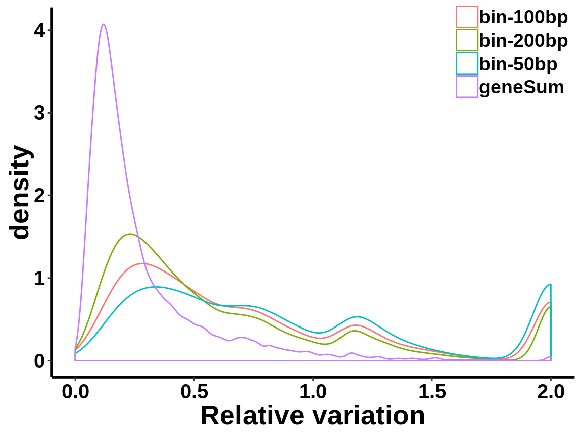

Compare MeRIP-seq IP data with regular RNA-seq data

var.coef <- function(x){sd(as.numeric(x))/mean(as.numeric(x))}

ip_coef_var <- t(apply(RADAR@ip_adjExpr_filtered,1,tapply,unlist(variable(RADAR)[,1]),var.coef))
ip_coef_var <- ip_coef_var[!apply(ip_coef_var,1,function(x){return(any(is.na(x)))}),]
#hist(c(ip_coef_var),main = "M14KO mouse liver\n m6A-IP",xlab = "within group coefficient of variation",breaks = 50)
###
gene_coef_var <-  t(apply(RADAR@geneSum,1,tapply,unlist(variable(RADAR)[,1]),var.coef))
gene_coef_var <- gene_coef_var[!apply(gene_coef_var,1,function(x){return(any(is.na(x)))}),]
#hist(c(gene_coef_var),main = "M14KO mouse liver\n RNA-seq",xlab = "within group coefficient of variation",breaks = 50)

coef_var <- list('RNA-seq'=c(gene_coef_var),'m6A-IP'=c(ip_coef_var))
nn<-sapply(coef_var, length)
rs<-cumsum(nn)
re<-rs-nn+1
grp <- factor(rep(names(coef_var), nn), levels=names(coef_var))
coef_var.df <- data.frame(coefficient_var = c(c(gene_coef_var),c(ip_coef_var)),label = grp)

ggplot(data = coef_var.df,aes(coefficient_var,colour = grp))+geom_density()+theme_bw() + theme(panel.border = element_blank(), panel.grid.major = element_blank(),
                   panel.grid.minor = element_blank(), axis.line = element_line(colour = "black",size = 1),
                   axis.title.x=element_text(size=20, face="bold", hjust=0.5,family = "arial"),
                   axis.title.y=element_text(size=20, face="bold", vjust=0.4, angle=90,family = "arial"),
                   legend.position = c(0.9,0.9),legend.title=element_blank(),legend.text = element_text(size = 18, face = "bold",family = "arial"),
                   axis.text.x = element_text(size = 15,face = "bold",family = "arial") ,axis.text.y = element_text(size = 15,face = "bold",family = "arial")  )+
  xlab("Coefficient of variation")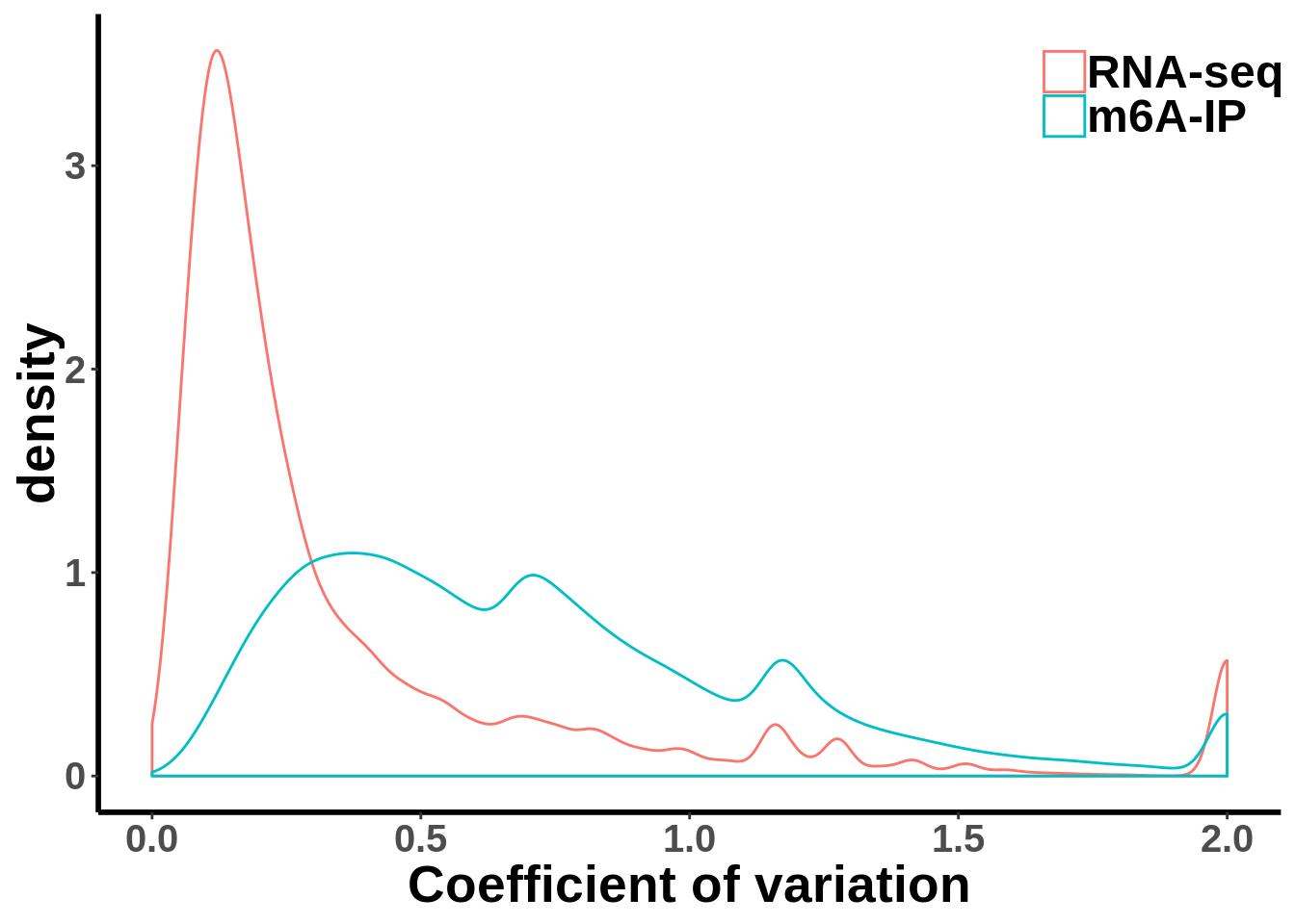

Check (within group) mean variance relationship of the data.

ip_var <- t(apply(RADAR@ip_adjExpr_filtered,1,tapply,unlist(variable(RADAR)[,1]),var))
#ip_var <- ip_coef_var[!apply(ip_var,1,function(x){return(any(is.na(x)))}),]
ip_mean <- t(apply(RADAR@ip_adjExpr_filtered,1,tapply,unlist(variable(RADAR)[,1]),mean))

###
gene_var <-  t(apply(RADAR@geneSum,1,tapply,unlist(variable(RADAR)[,1]),var))
#gene_var <- gene_var[!apply(gene_var,1,function(x){return(any(is.na(x)))}),]
gene_mean <- t(apply(RADAR@geneSum,1,tapply,unlist(variable(RADAR)[,1]),mean))

all_var <- list('RNA-seq'=c(gene_var),'m6A-IP'=c(ip_var))
nn<-sapply(all_var, length)
rs<-cumsum(nn)
re<-rs-nn+1
group <- factor(rep(names(all_var), nn), levels=names(all_var))
all_var.df <- data.frame(variance = c(c(gene_var),c(ip_var)),mean= c(c(gene_mean),c(ip_mean)),label = group)

ggplot(data = all_var.df,aes(x=mean,y=variance,colour = group,shape = group) )+geom_point(size = I(0.2))+stat_smooth(se = T,show.legend = F)+stat_smooth(se = F)+theme_bw() +xlab("Mean")+ ylab("Variance") + theme(panel.border = element_blank(), panel.grid.major = element_blank(),
                   panel.grid.minor = element_blank(), axis.line = element_line(colour = "black",size = 1),
                   axis.title.x=element_text(size=22, face="bold", hjust=0.5,family = "arial"),
                   axis.title.y=element_text(size=22, face="bold", vjust=0.4, angle=90,family = "arial"),
                   legend.position = c(0.85,0.95),legend.title=element_blank(),legend.text = element_text(size = 20, face = "bold",family = "arial"),
                   axis.text.x = element_text(size = 15,face = "bold",family = "arial") ,axis.text.y = element_text(size = 15,face = "bold",family = "arial")) +
  scale_x_continuous(limits = c(0,10000))+scale_y_continuous(limits = c(0,7e6),labels = scales::scientific)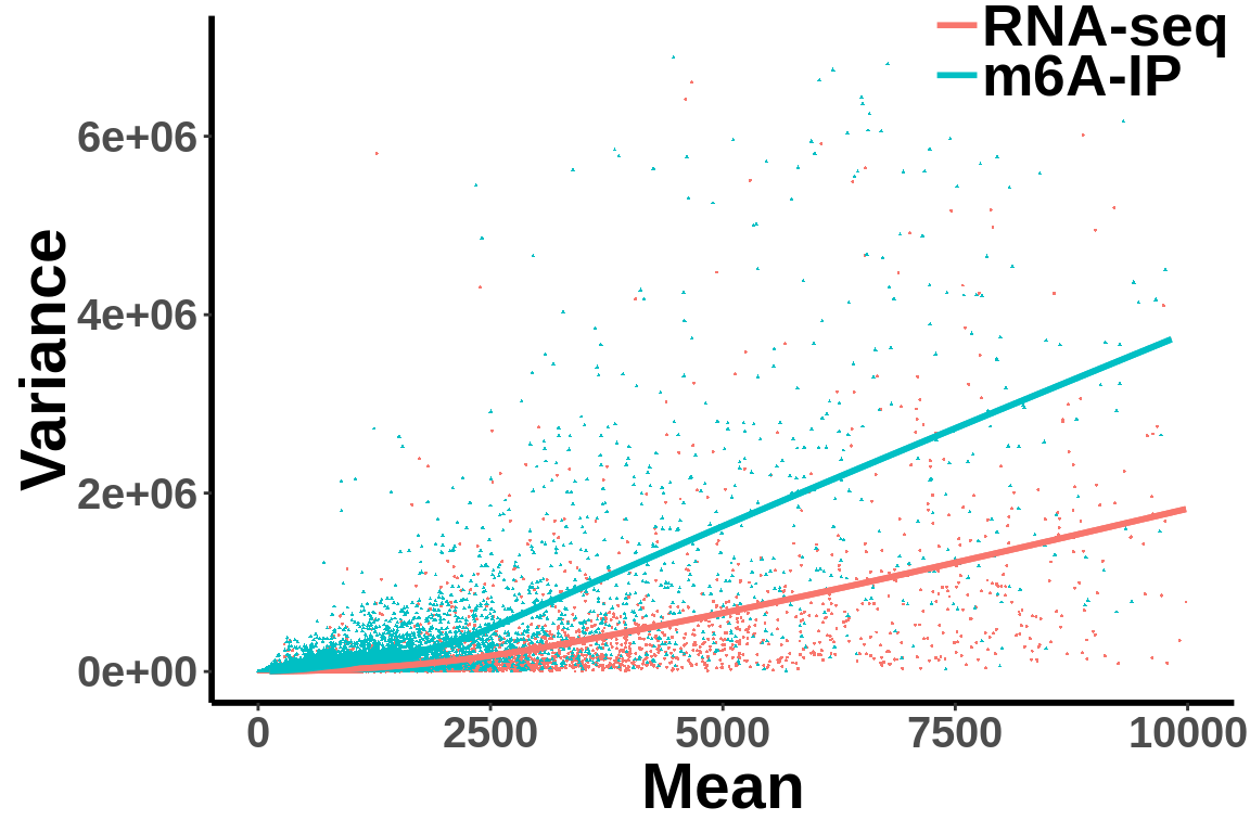

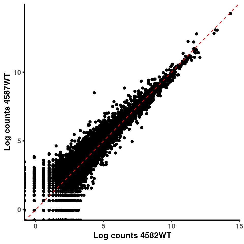
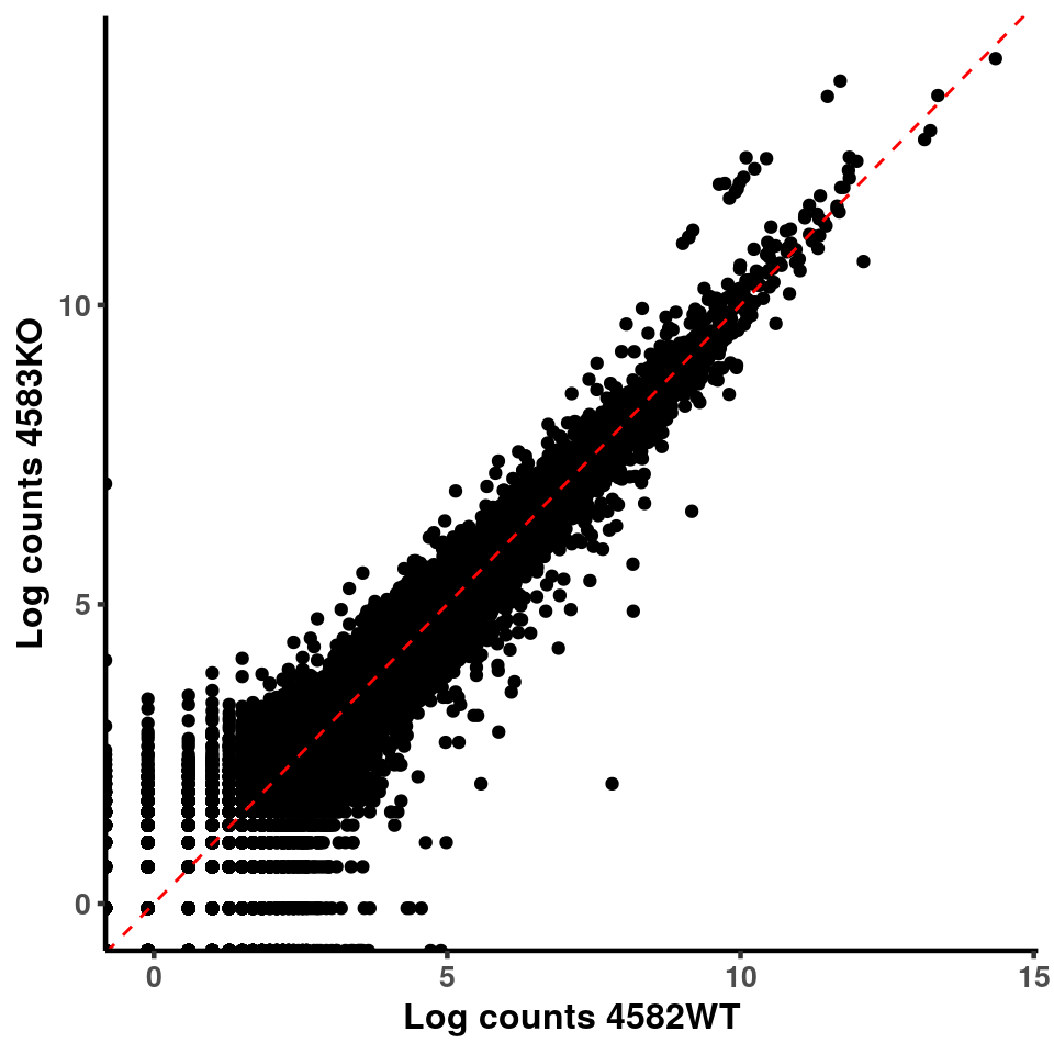
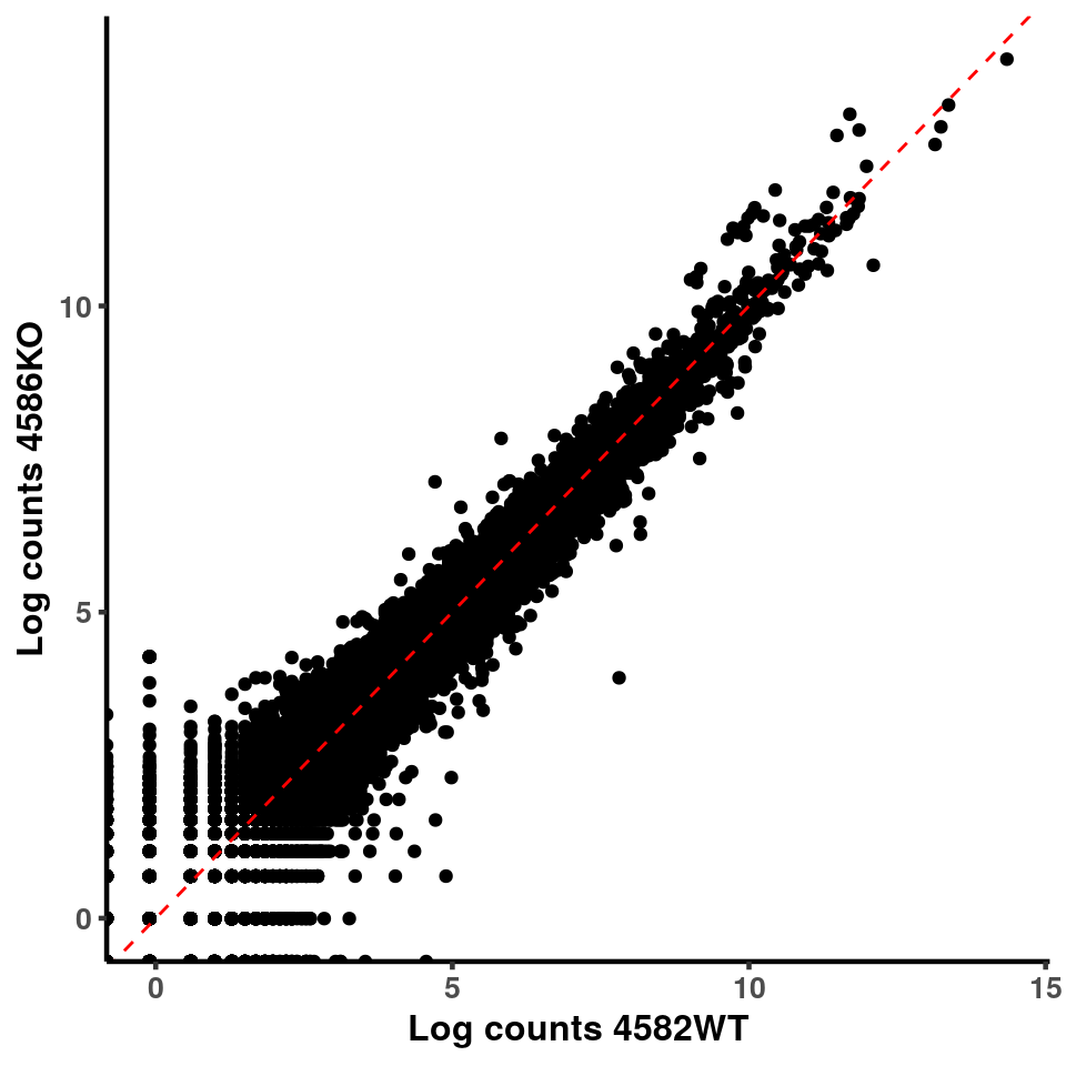
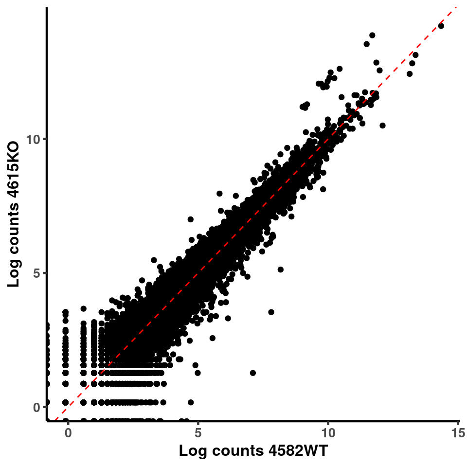
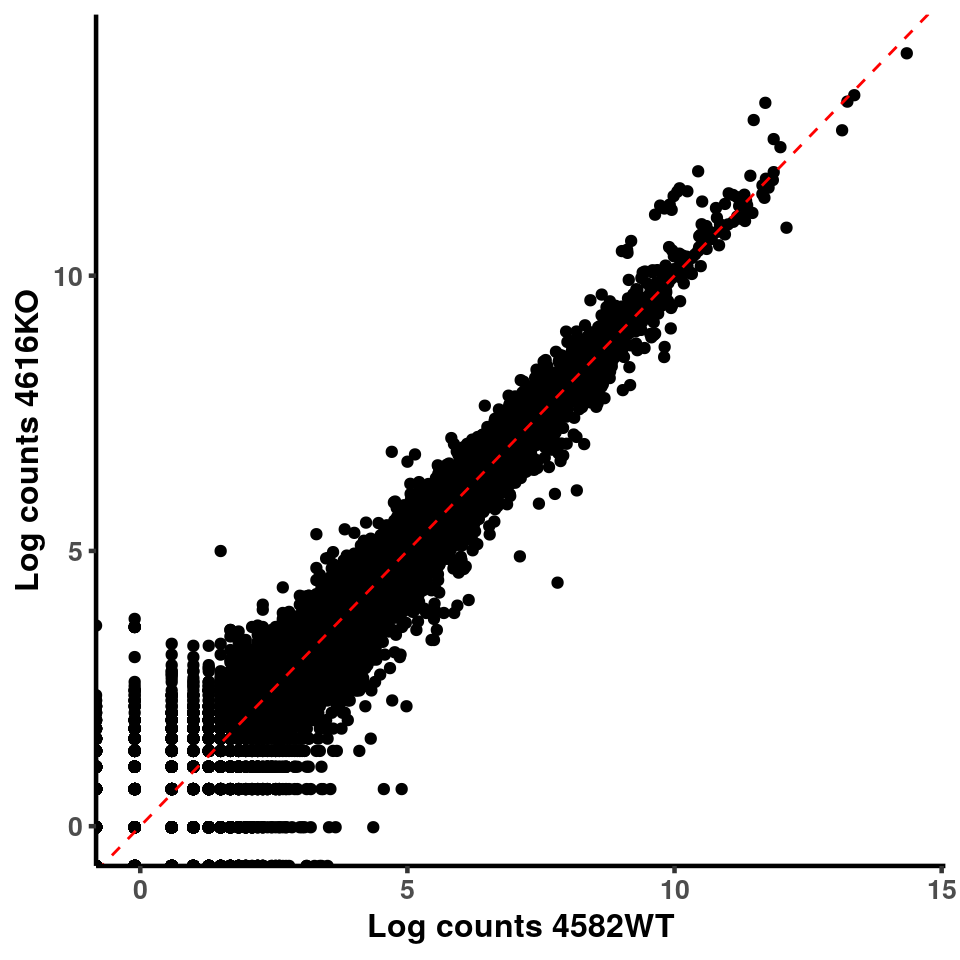
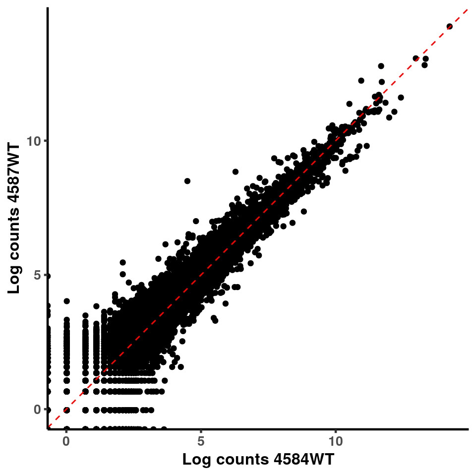
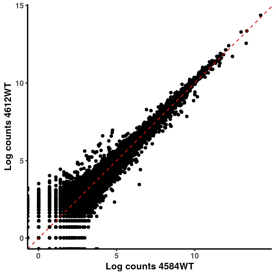
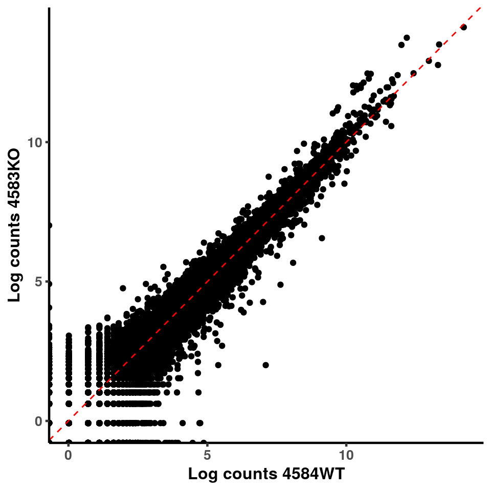
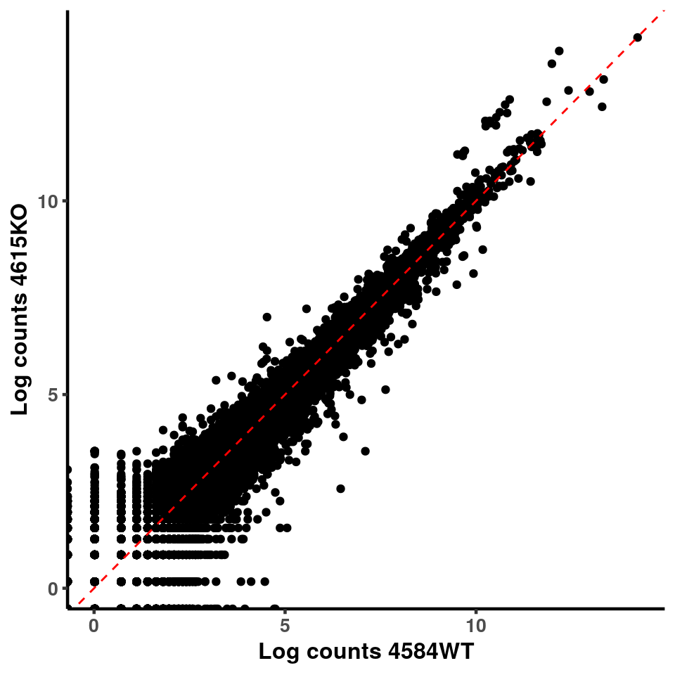
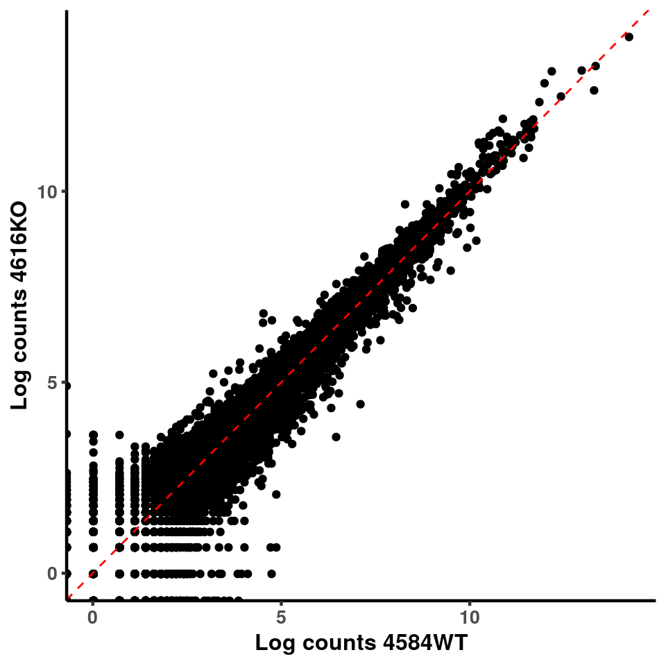
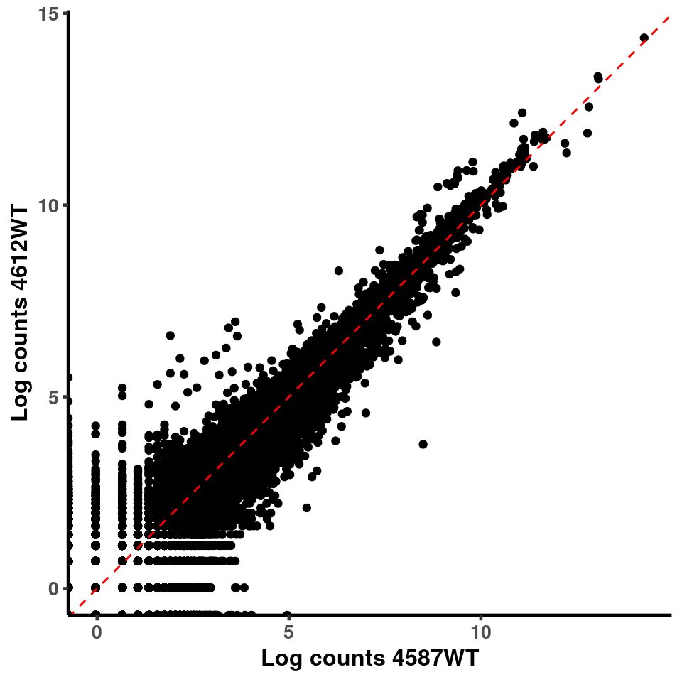
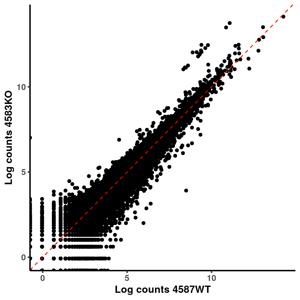
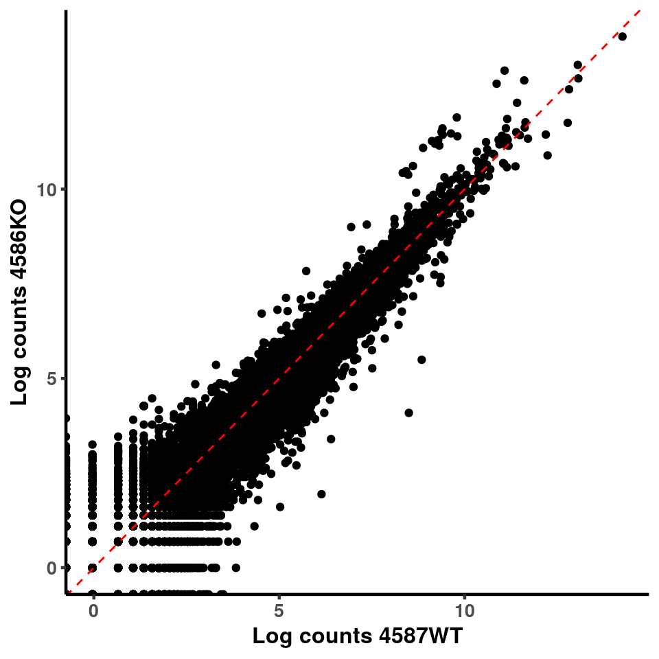
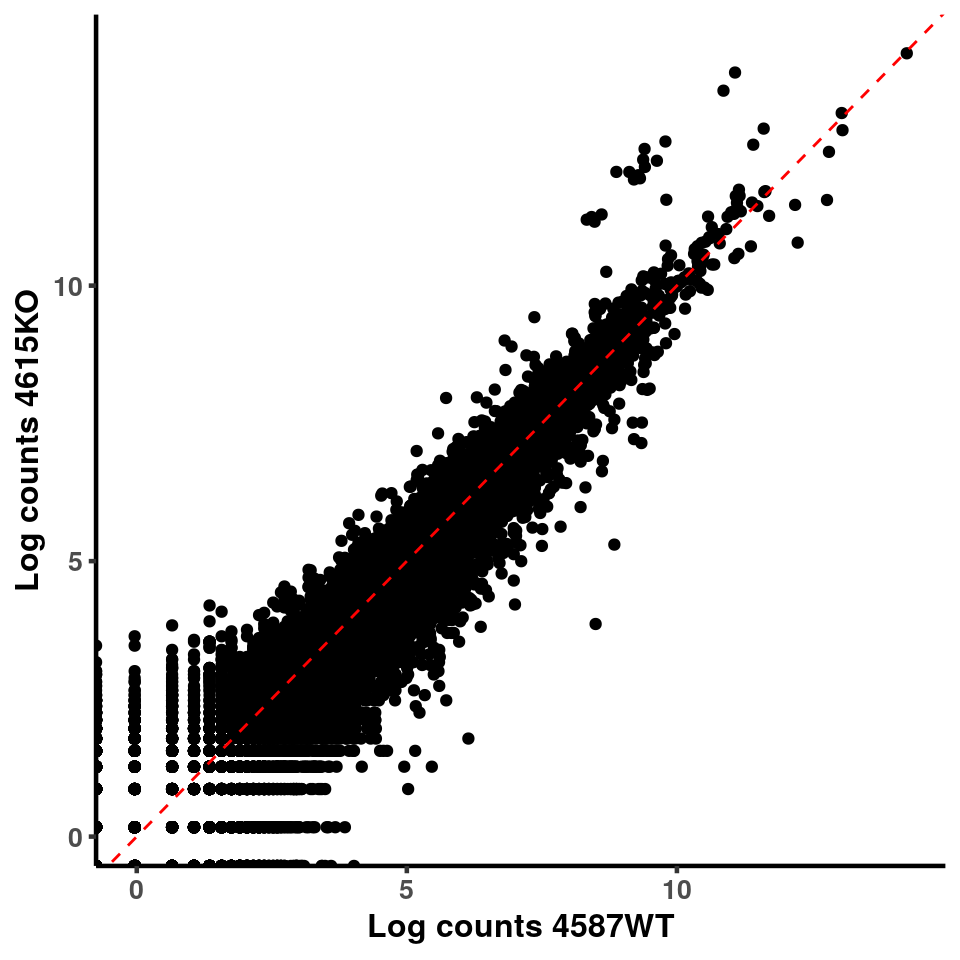
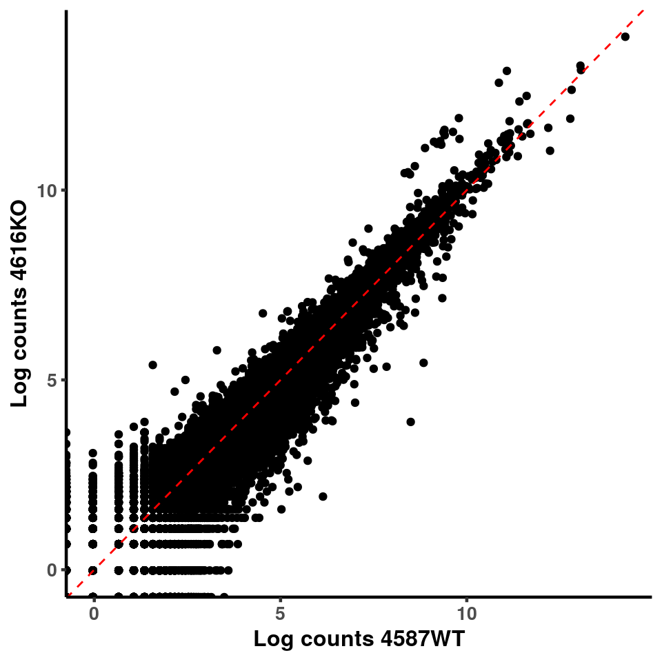
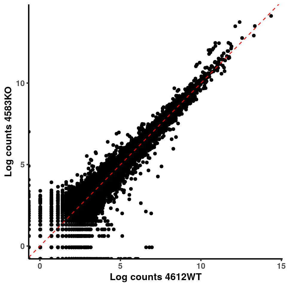
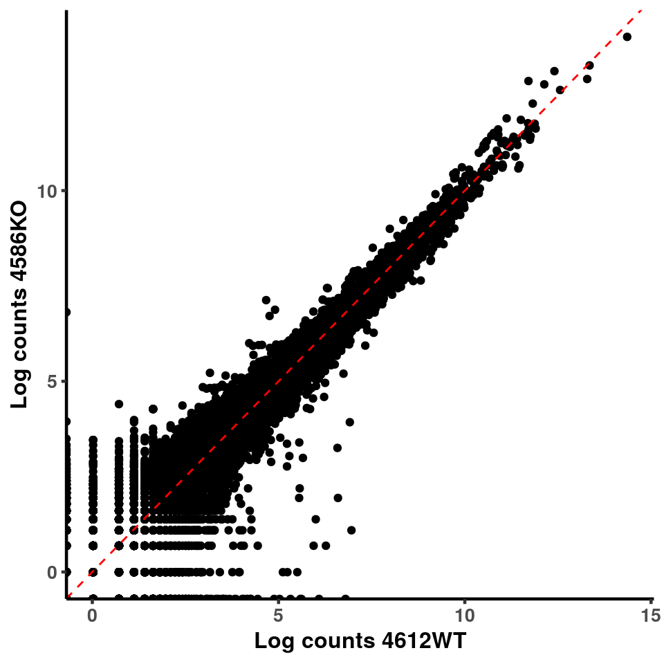
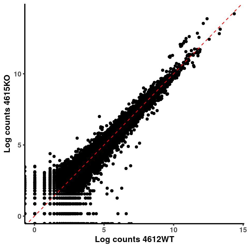
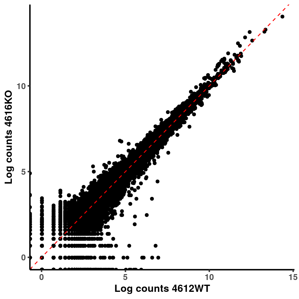
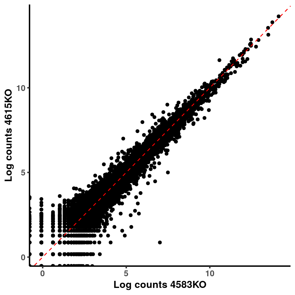
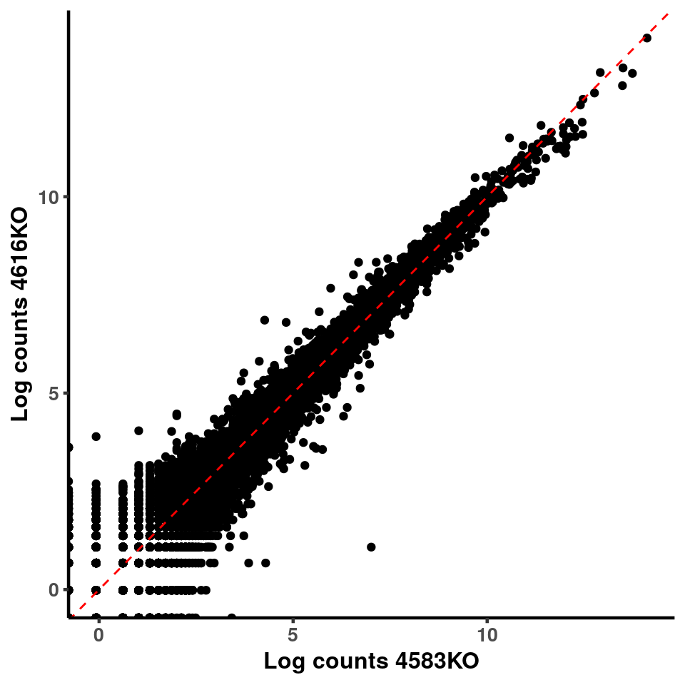
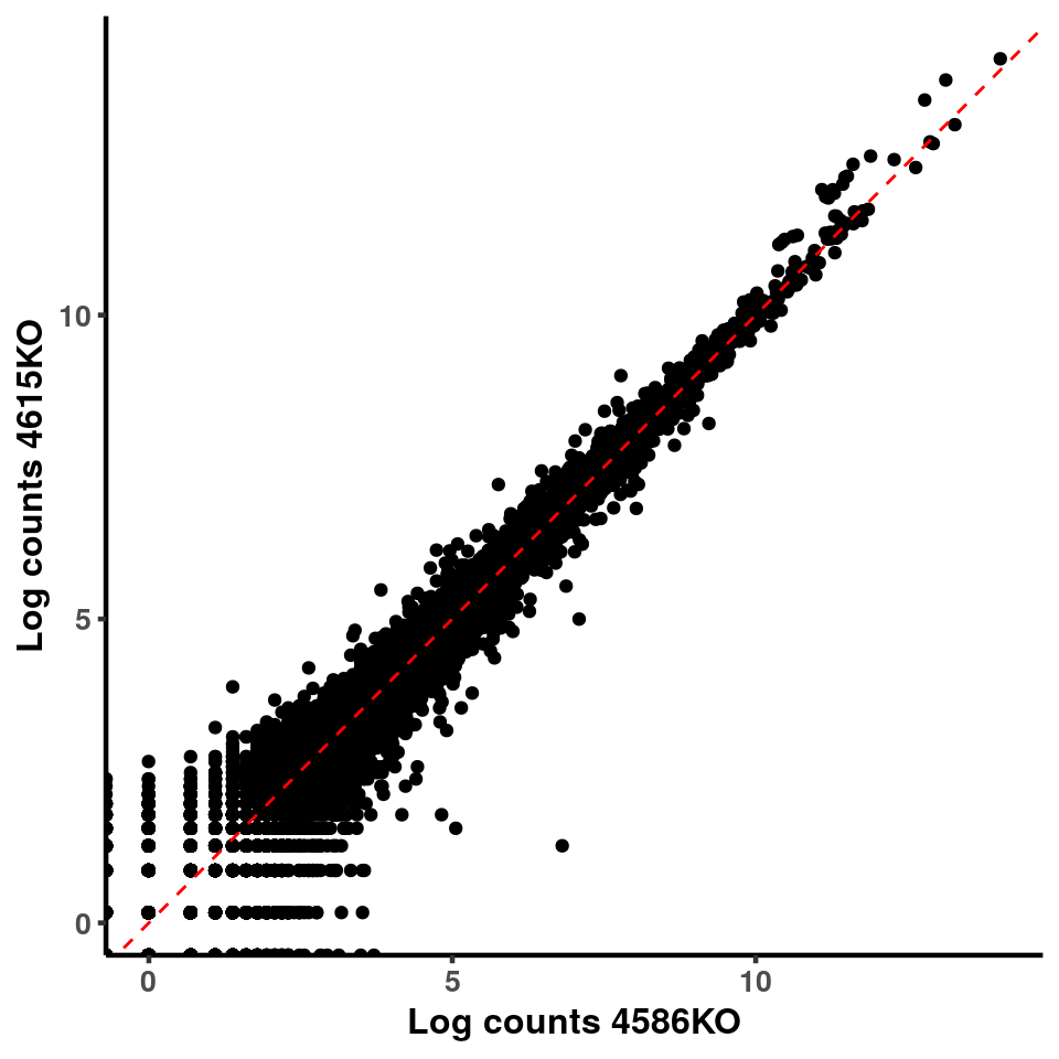
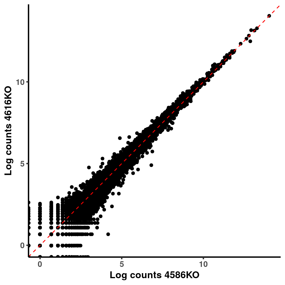
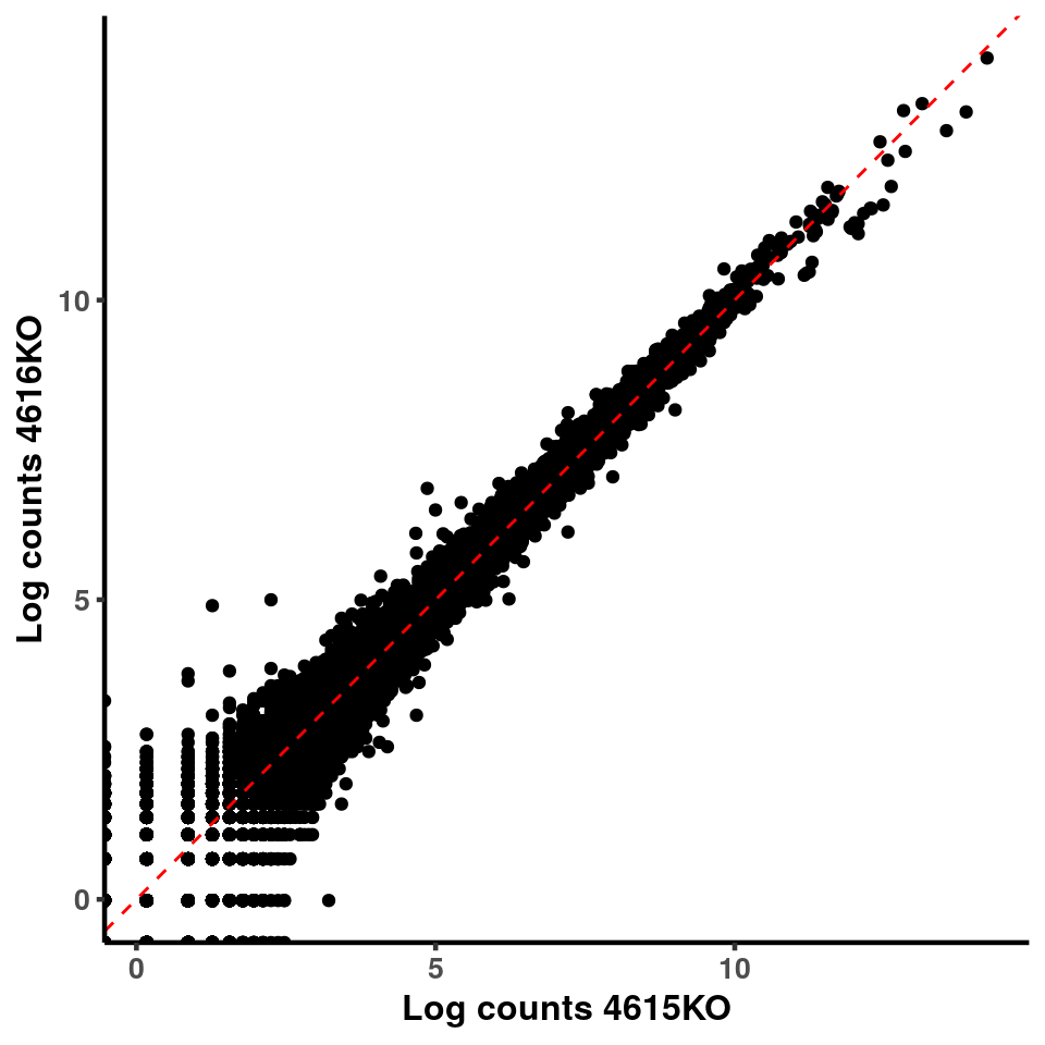
inputCount <- as.data.frame(RADAR@reads[,1:length(RADAR@samplenames)])
logInputCount <- as.data.frame(log( RADAR@geneSum  )  )
for(xx in 1:7){
  for(x in (xx+1):8){
  p <- ggplot(logInputCount, aes(x = logInputCount[,xx] , y = logInputCount[,x] ))+geom_point()+geom_abline(intercept = 0,slope = 1, lty = 2, colour = "red")+xlab(paste("Log counts",colnames(logInputCount)[xx],  sep = " ") )+ylab(paste("Log counts",colnames(logInputCount)[x],sep = " ") )+theme_classic(base_line_size = 0.8)+theme(axis.title = element_text(size = 12,face = "bold"), axis.text =  element_text(size = 10,face = "bold") )
  print(p)
  }
}

ggplot(logInputCount, aes(x = `4583KO` , y = `4587WT` ))+geom_point()+geom_abline(intercept = 0,slope = 1, lty = 2, colour = "red")+xlab(paste("Log counts 4583KO") )+ylab(paste("Log counts 4587WT") )+theme_classic(base_line_size = 0.8)+theme(axis.title = element_text(size = 12,face = "bold"), axis.text =  element_text(size = 10,face = "bold") )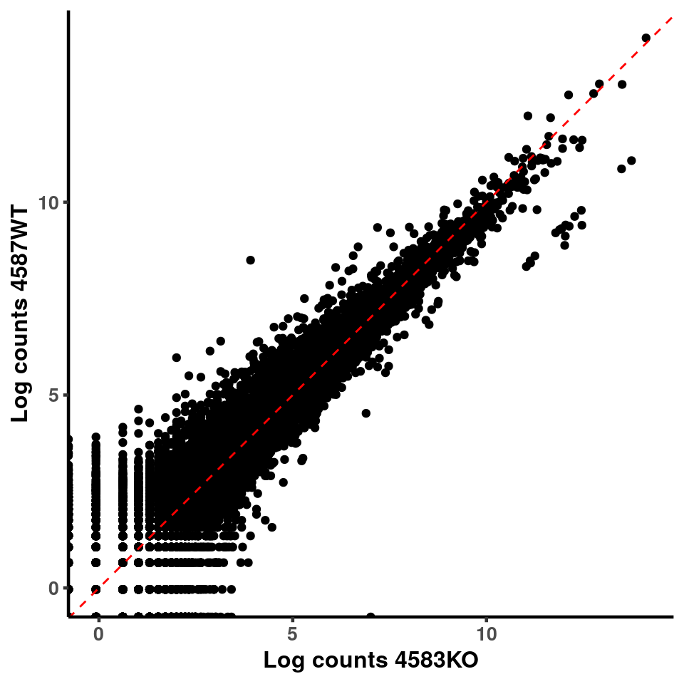

ggplot(logInputCount, aes(x = `4615KO` , y = `4584WT` ))+geom_point()+geom_abline(intercept = 0,slope = 1, lty = 2, colour = "red")+xlab(paste("Log counts 4615KO") )+ylab(paste("Log counts 4584WT") )+theme_classic(base_line_size = 0.8)+theme(axis.title = element_text(size = 12,face = "bold"), axis.text =  element_text(size = 10,face = "bold") )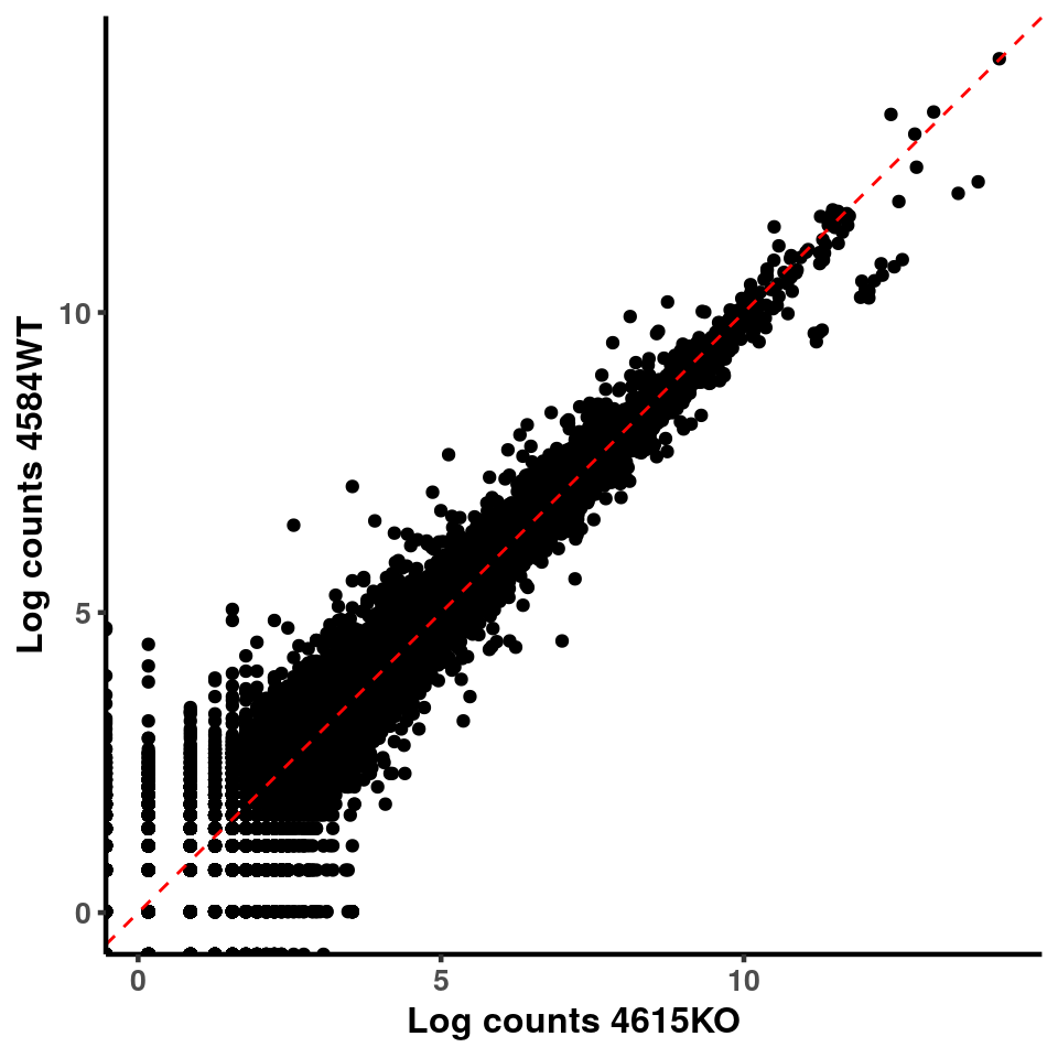

PCA analysis

After geting the filtered IP read count for testing, we can first use PCA analysis to check unkown variation.

top_bins <- RADAR@ip_adjExpr_filtered[order(rowMeans(RADAR@ip_adjExpr_filtered))[1:15000],]

We plot PCA colored by WT vs KO

plotPCAfromMatrix(top_bins,group = unlist(variable(RADAR)[,1]) )+scale_color_discrete(name = "Group")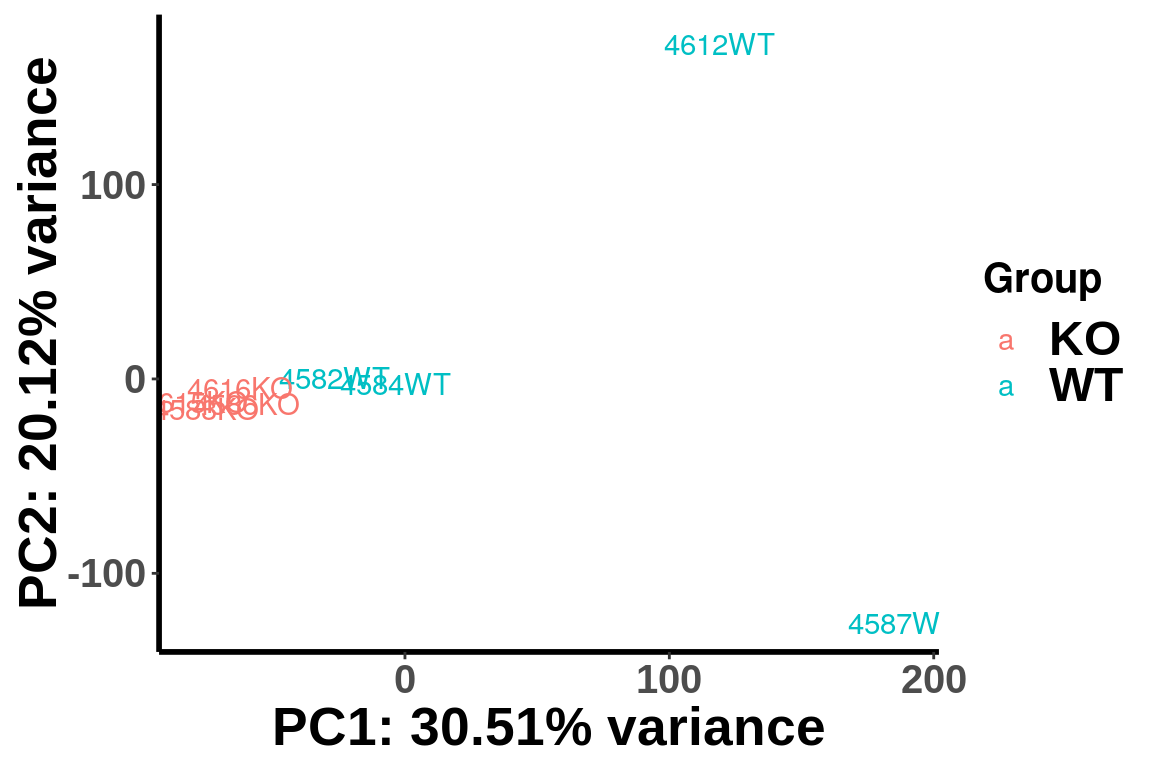

Run RADAR test

RADAR <-  diffIP_parallel(RADAR,thread = 25  , fdrBy = "fdr")
RADAR_pos <-  diffIP_parallel(RADAR_pos,thread = 25 ,fdrBy = "fdr")

Other method

## fisher's exact test
fisherTest <- function( control_ip, treated_ip, control_input, treated_input, thread ){
  registerDoParallel(cores = thread)
  testResult <- foreach(i = 1:nrow(control_ip) , .combine = rbind )%dopar%{
    tmpTest <- fisher.test( cbind( c( rowSums(treated_ip)[i], rowSums(treated_input)[i] ), c( rowSums(control_ip)[i], rowSums(control_input)[i] ) ), alternative = "two.sided" )
    data.frame( logFC = log(tmpTest$estimate), pvalue =  tmpTest$p.value )
  }
  rm(list=ls(name=foreach:::.foreachGlobals), pos=foreach:::.foreachGlobals)
  testResult$fdr <- p.adjust(testResult$pvalue, method = "fdr")
  return(testResult)
}

## wrapper for the MetDiff test
MeTDiffTest <-  function( control_ip, treated_ip, control_input, treated_input, thread = 1 ){
  registerDoParallel(cores = thread)
  testResult <- foreach(i = 1:nrow(control_ip) , .combine = rbind )%dopar%{
    x <- t( as.matrix(control_ip[i,]) )
    y <- t( as.matrix(control_input[i,]) )
    xx <- t( as.matrix(treated_ip[i,]) )
    yy <- t( as.matrix(treated_input[i,]) )
    xxx = cbind(x,xx)
    yyy = cbind(y,yy)
    
    logl1 <- MeTDiff:::.betabinomial.lh(x,y+1)
    logl2 <- MeTDiff:::.betabinomial.lh(xx,yy+1)
    logl3 <- MeTDiff:::.betabinomial.lh(xxx,yyy+1)
    tst <- (logl1$logl+logl2$logl-logl3$logl)*2
    pvalues <- 1 - pchisq(tst,2)
    log.fc <- log( (sum(xx)+1)/(1+sum(yy)) * (1+sum(y))/(1+sum(x)) ) 
    
    data.frame( logFC = log.fc, pvalue =  pvalues )
  }
  rm(list=ls(name=foreach:::.foreachGlobals), pos=foreach:::.foreachGlobals)
  testResult$fdr <- p.adjust(testResult$pvalue, method = "fdr")
  return(testResult)
}


Bltest <- function(control_ip, treated_ip, control_input, treated_input){
  control_ip_total <- sum(colSums(control_ip))
  control_input_total <- sum(colSums(control_input))
  treated_ip_total <- sum(colSums(treated_ip))
  treated_input_total <- sum(colSums(treated_input))
  
  tmpResult <- do.call(cbind.data.frame, exomePeak::bltest(rowSums(control_ip), rowSums(control_input),rowSums(treated_ip),rowSums(treated_input),control_ip_total, control_input_total, treated_ip_total,  treated_input_total) ) 
  return( data.frame(logFC = tmpResult[,"log.fc"], pvalue = exp(tmpResult[,"log.p"]), fdr = exp(tmpResult$log.fdr) ) )
}

In order to compare performance of other method on this data set, we run other three methods on default mode on this dataset.

filteredBins <- rownames(RADAR@ip_adjExpr_filtered) 

 Metdiff.res <-MeTDiffTest(control_ip = round( RADAR@norm.ip[filteredBins,1:4] ) ,
                        treated_ip = round( RADAR@norm.ip[filteredBins,5:8] ),
                        control_input = round( RADAR@norm.input[filteredBins,1:4] ),
                        treated_input = round( RADAR@norm.input[filteredBins,5:8] ) , thread = 20)


  QNB.res <- QNB::qnbtest(control_ip = round( RADAR@norm.ip[filteredBins,1:4] ) ,
                        treated_ip = round( RADAR@norm.ip[filteredBins,5:8] ),
                        control_input = round( RADAR@norm.input[filteredBins,1:4] ),
                        treated_input = round( RADAR@norm.input[filteredBins,5:8] ) ,plot.dispersion = FALSE )

  fisher.res <- fisherTest(control_ip = round( RADAR@norm.ip[filteredBins,1:4] ) ,
                        treated_ip = round( RADAR@norm.ip[filteredBins,5:8] ),
                        control_input = round( RADAR@norm.input[filteredBins,1:4] ),
                        treated_input = round( RADAR@norm.input[filteredBins,5:8] ) )
  
  exomePeak.res <- Bltest(control_ip = round( RADAR@norm.ip[filteredBins,1:4] ) ,
                        treated_ip = round( RADAR@norm.ip[filteredBins,5:8] ),
                        control_input = round( RADAR@norm.input[filteredBins,1:4] ),
                        treated_input = round( RADAR@norm.input[filteredBins,4:8] ) )

Compare distribution of p value.

pvalues <- data.frame(pvalue = c(RADAR@test.est[,"p_value"],Metdiff.res$pvalue,QNB.res$pvalue,fisher.res$pvalue, exomePeak.res$pvalue ),
                      method = factor(rep(c("RADAR","MeTDiff","QNB","Fisher","exomePeak"),c(length(RADAR@test.est[,"p_value"]),
                                                                       length(Metdiff.res$pvalue),
                                                                       length(QNB.res$pvalue),
                                                                       length(fisher.res$pvalue),
                                                                       length(exomePeak.res$pvalue)
                                                                       )
                                          ),levels =c("RADAR","MeTDiff","QNB","Fisher","exomePeak")
                                   )
                      )
ggplot(pvalues, aes(x = pvalue))+geom_histogram(breaks = seq(0,1,0.04),col=I("black"))+facet_grid(.~method)+theme_bw()+xlab("p-value")+theme( axis.title =  element_text(size = 22, face = "bold"),strip.text = element_text(size = 25, face = "bold"),axis.text.x = element_text(size = 18, face = "bold",colour = "black"),axis.text.y = element_text(size = 15, face = "bold",colour = "black",angle = 90),panel.grid = element_blank(), axis.line = element_line(size = 0.7 ,colour = "black"),axis.ticks = element_line(colour = "black"), panel.spacing = unit(0.4, "lines") )+ scale_x_continuous(breaks = seq(0,1,0.2),labels=function(x) sprintf("%.1f", x))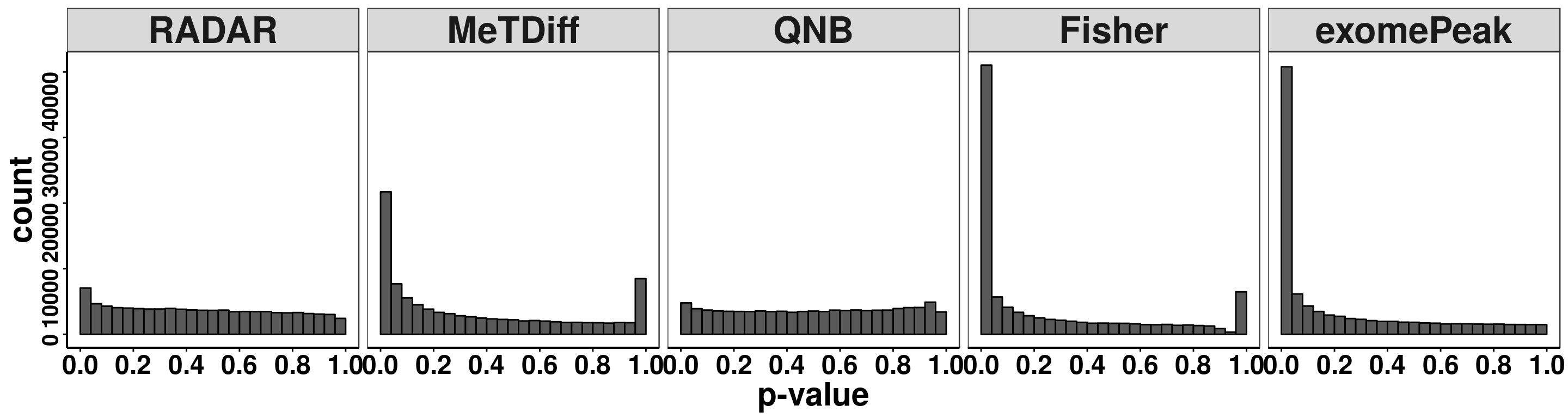

Compare adjusting expression level by geneSum vs. bin read counts.

tmp <- hist(c(RADAR_pos@test.est[,"p_value"]),plot = F)
tmp$counts <- tmp$counts*(nrow(RADAR@ip_adjExpr_filtered)/nrow(RADAR_pos@ip_adjExpr_filtered))
hist(RADAR@test.est[,"p_value"],main = "RADAR",xlab = "p value",col =rgb(1,0,0,0.4),cex.main = 2.5,cex.axis =2,cex.lab=2, ylim = c(0,max(hist(RADAR@test.est[,"p_value"],plot = F)$counts,tmp$counts)) )
plot(tmp,col=rgb(0,0,1,0.5),add = T)
axis(side = 1, lwd = 1,cex.axis =2)
axis(side = 2, lwd = 1,cex.axis =2)
legend("topright", c("By geneSum", "By position"), col=c(rgb(1,0,0,0.4), rgb(0,0,1,0.5)), lwd = 10,bty="n",text.font = 2)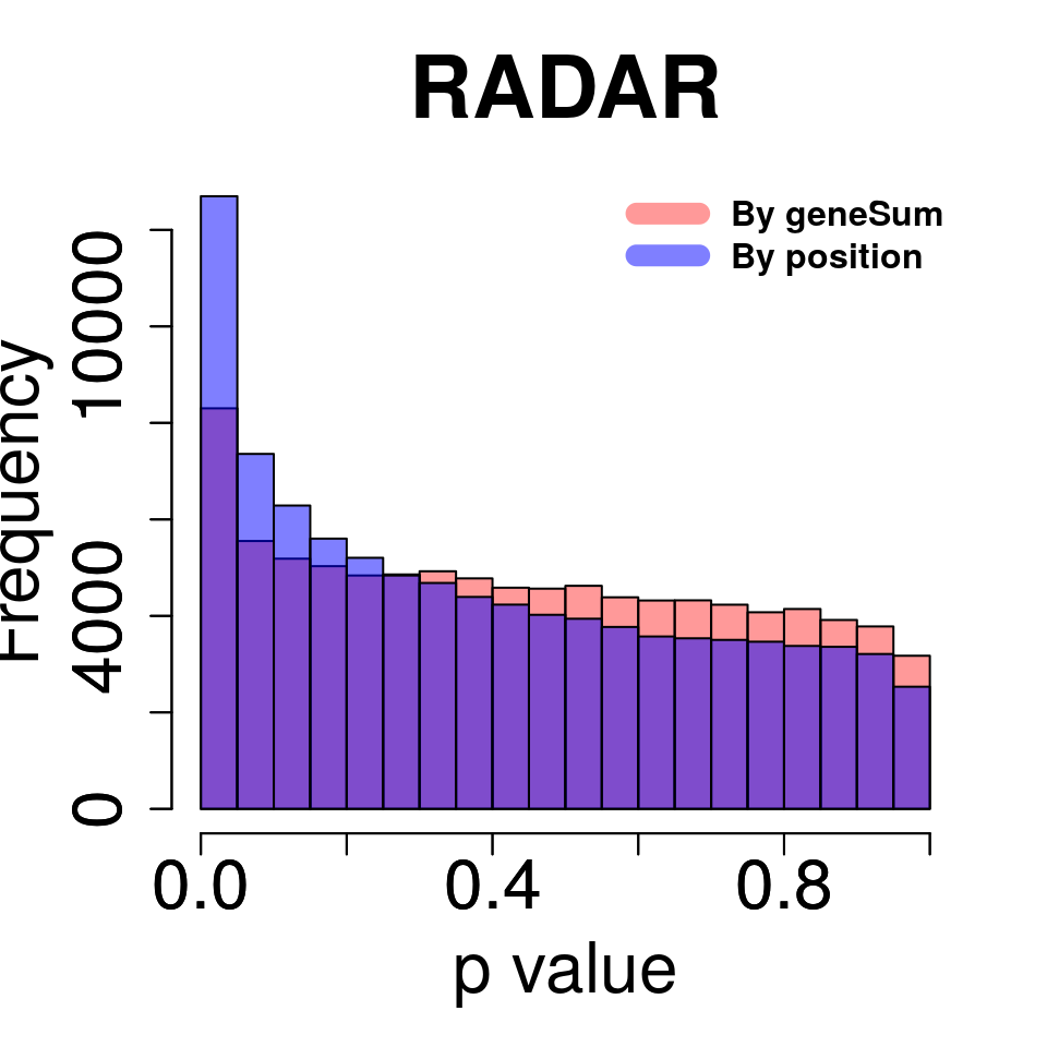

Permutation Test

radar_permuted_P <-NULL
metdiff_permuted_P <- NULL
qnb_permuted_P <- NULL
fisher_permuted_P <- NULL
exomePeak_permute_P <- NULL

set.seed(2)
for(i in 1:15){
  
  permute_X <- variable(RADAR)[,1]
  permute_X[sample(1:4, 2 )] <- "KO"
  permute_X[sample(5:8, 2 )] <- "WT"
  RADAR_permute <- RADAR
  variable(RADAR_permute) <- data.frame(condition = permute_X  )
    
  radar_permute <- diffIP_parallel( RADAR_permute , thread = 20 )@test.est[,"p_value"]
  
  metdiff_permute <-MeTDiffTest( control_ip = round( RADAR@norm.ip[filteredBins ,(which(permute_X == "WT" ) )] ),
                                 treated_ip = round( RADAR@norm.ip[filteredBins,(which(permute_X == "KO" ) )] ),
                                 control_input = round( RADAR@norm.input[filteredBins,which(permute_X == "WT" )] ),
                                 treated_input = round( RADAR@norm.input[filteredBins,which(permute_X == "KO" )] ) ,
                                 thread = 25)$pvalue
  
  qnb_permute <- QNB::qnbtest(control_ip = round( RADAR@norm.ip[filteredBins ,(which(permute_X == "WT" ) )] ),
                              treated_ip = round( RADAR@norm.ip[filteredBins,(which(permute_X == "KO" ) )] ),
                              control_input = round( RADAR@norm.input[filteredBins,which(permute_X == "WT" )] ),
                              treated_input = round( RADAR@norm.input[filteredBins,which(permute_X == "KO" )] ),
                              plot.dispersion = FALSE)$pvalue
  
  fisher_permute <- fisherTest( control_ip = round( RADAR@norm.ip[filteredBins ,(which(permute_X == "WT" ) )] ),
                                treated_ip = round( RADAR@norm.ip[filteredBins,(which(permute_X == "KO" ) )] ),
                                control_input = round( RADAR@norm.input[filteredBins,which(permute_X == "wT" )] ),
                                treated_input = round( RADAR@norm.input[filteredBins,which(permute_X == "KO" )] )  ,
                                thread = 25
                               )$pvalue
  
  exomePeak_permute <- Bltest( control_ip = round( RADAR@norm.ip[filteredBins ,(which(permute_X == "WT" ) )] ),
                               treated_ip = round( RADAR@norm.ip[filteredBins,(which(permute_X == "KO" ) )] ),
                               control_input = round( RADAR@norm.input[filteredBins,which(permute_X == "WT" )] ),
                               treated_input = round( RADAR@norm.input[filteredBins,which(permute_X == "KO" )] )
                              )$pvalue
                    
  radar_permuted_P <- cbind(radar_permuted_P, radar_permute)
  metdiff_permuted_P <- cbind(metdiff_permuted_P, metdiff_permute)
  qnb_permuted_P <- cbind(qnb_permuted_P,qnb_permute)
  fisher_permuted_P <- cbind(fisher_permuted_P, fisher_permute)
  exomePeak_permute_P <- cbind(exomePeak_permute_P, exomePeak_permute)
  
}

for( i in 1:ncol(radar_permuted_P)){
par(mfrow=c(1,5))
hist(RADAR@test.est[,"p_value"], col =rgb(1,0,0,0.4),main = "RADAR", xlab = "p value",cex.main = 2.5,cex.axis =2,cex.lab=2)
hist(radar_permuted_P[,i],col=rgb(0,0,1,0.5),add = T)
legend("topright", c("Original", "Permuted"), col=c(rgb(1,0,0,0.4), rgb(0,0,1,0.5)), lwd = 10,bty="n")
hist(Metdiff.res$pvalue, col =rgb(1,0,0,0.4),main = "MeTdiff",xlab = "p value",cex.main = 2.5,cex.axis =2,cex.lab=2)
hist(metdiff_permuted_P[,i],col=rgb(0,0,1,0.5),add = T)
legend("topright", c("Original", "Permuted"), col=c(rgb(1,0,0,0.4), rgb(0,0,1,0.5)), lwd = 10,bty="n")
hist(QNB.res$pvalue, col =rgb(1,0,0,0.4),main = "QNB",xlab = "p value",cex.main = 2.5,cex.axis =2,cex.lab=2)
hist(qnb_permuted_P[,i],col=rgb(0,0,1,0.5),add = T)
legend("topright", c("Original", "Permuted"), col=c(rgb(1,0,0,0.4), rgb(0,0,1,0.5)), lwd = 10,bty="n")
hist(fisher.res$pvalue, col =rgb(1,0,0,0.4),main = "Fisher",xlab = "p value",cex.main = 2.5,cex.axis =2,cex.lab=2)
hist(fisher_permuted_P[,i],col=rgb(0,0,1,0.5),add = T)
legend("topright", c("Original", "Permuted"), col=c(rgb(1,0,0,0.4), rgb(0,0,1,0.5)), lwd = 10,bty="n")
hist(exomePeak.res$pvalue, col =rgb(1,0,0,0.4),main = "exomePeak",xlab = "p value",cex.main = 2.5,cex.axis =2,cex.lab=2)
hist(exomePeak_permute_P[,i],col=rgb(0,0,1,0.5),add = T)
legend("topright", c("Original", "Permuted"), col=c(rgb(1,0,0,0.4), rgb(0,0,1,0.5)), lwd = 10,bty="n")

}

par(mfrow=c(1,5))

y.scale <- max(hist(c(fisher_permuted_P) ,plot = F)$counts)/15

hist(RADAR@test.est[,"p_value"], col =rgb(1,0,0,0.4),main = "RADAR", xlab = "p value",font=2, cex.lab=2.5, cex.axis = 1.5 , font.lab=2 ,cex.main = 3, lwd = 3,  ylim = c(0,y.scale) )
tmp <- hist(c(radar_permuted_P),plot = F)
tmp$counts <- tmp$counts/15
plot(tmp,col=rgb(0,0,1,0.5),add = T)
legend("topright", c("Original", "Permuted"), col=c(rgb(1,0,0,0.4), rgb(0,0,1,0.5)), lwd = 12,bty="n",text.font = 2, cex = 1.5)
 

tmp <- hist(c(metdiff_permuted_P),plot = F)
tmp$counts <- tmp$counts/15
hist(Metdiff.res$pvalue, col =rgb(1,0,0,0.4),main = "MeTDiff",xlab = "p value" ,font=2, cex.lab=2.5, cex.axis = 1.5 , font.lab=2 ,cex.main = 3, lwd = 3, ylim = c(0,y.scale) )
plot(tmp,col=rgb(0,0,1,0.5),add = T)
legend("topright", c("Original", "Permuted"), col=c(rgb(1,0,0,0.4), rgb(0,0,1,0.5)), lwd = 12,bty="n",text.font = 2, cex = 1.5)

hist(QNB.res$pvalue, col =rgb(1,0,0,0.4),main = "QNB",xlab = "p value",font=2, cex.lab=2.5, cex.axis = 1.5 , font.lab=2 ,cex.main = 3,lwd = 3,ylim = c(0,y.scale))
tmp <- hist(c(qnb_permuted_P),plot = F)
tmp$counts <- tmp$counts/15
plot(tmp,col=rgb(0,0,1,0.5),add = T)
legend("topright", c("Original", "Permuted"), col=c(rgb(1,0,0,0.4), rgb(0,0,1,0.5)), lwd = 12,bty="n",text.font = 2, cex = 1.5)

hist(fisher.res$pvalue, col =rgb(1,0,0,0.4),main = "Fisher",xlab = "p value",font=2, cex.lab=2.5, cex.axis = 1.5 , font.lab=2 ,cex.main = 3,lwd = 3,ylim = c(0,y.scale))
tmp <- hist(c(fisher_permuted_P),plot = F)
tmp$counts <- tmp$counts/15
plot(tmp,col=rgb(0,0,1,0.5),add = T)
legend("topright", c("Original", "Permuted"), col=c(rgb(1,0,0,0.4), rgb(0,0,1,0.5)), lwd = 12,bty="n",text.font = 2, cex = 1.5)


hist(exomePeak.res$pvalue, col =rgb(1,0,0,0.4),main = "exomePeak",xlab = "p value",font=2, cex.lab=2.5, cex.axis = 1.5 , font.lab=2 ,cex.main = 3,lwd = 3,ylim = c(0,y.scale))
tmp <- hist(c(exomePeak_permute_P),plot = F)
tmp$counts <- tmp$counts/15
plot(tmp,col=rgb(0,0,1,0.5),add = T)
legend("topright", c("Original", "Permuted"), col=c(rgb(1,0,0,0.4), rgb(0,0,1,0.5)), lwd = 12,bty="n",text.font = 2, cex = 1.5)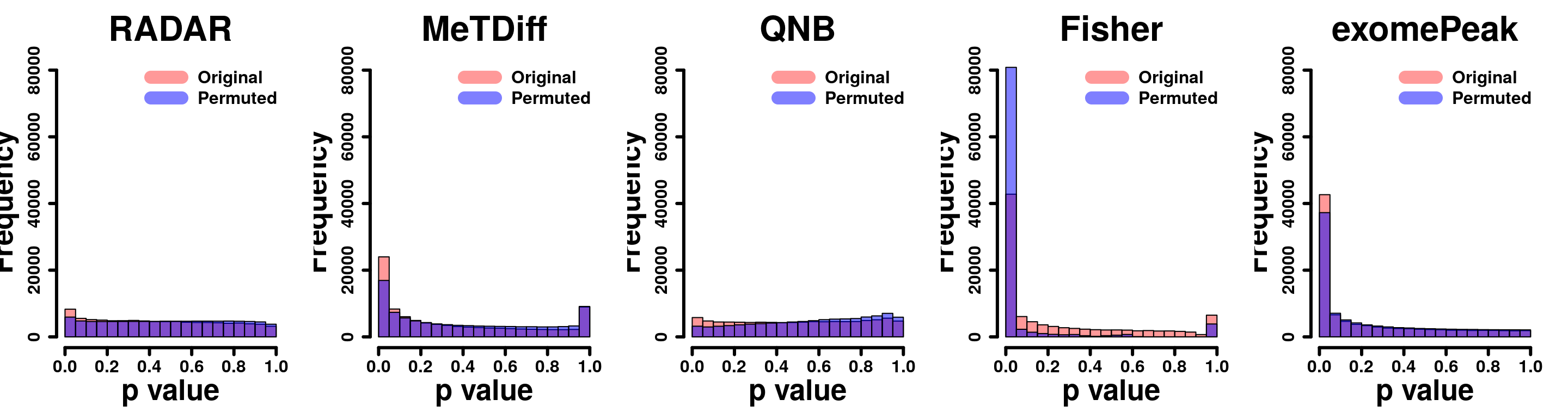

Permutation by position

radar_permuted_P_pos <-NULL

set.seed(2)
for(i in 1:15){
  
  permute_X <- variable(RADAR)[,1]
  permute_X[sample(1:4, 2 )] <- "KO"
  permute_X[sample(5:8, 2 )] <- "WT"
  RADAR_permute <- RADAR_pos
  variable(RADAR_permute) <- data.frame(condition = permute_X  )
    
  radar_permute <- diffIP_parallel( RADAR_permute , thread = 20 )@test.est[,"p_value"]
  
  
  radar_permuted_P_pos <- cbind(radar_permuted_P_pos, radar_permute)
}

par(mfrow=c(1,2))


y.scale <- max(hist( RADAR_pos@test.est[,"p_value"] ,plot = F)$counts)+1000

hist(RADAR@test.est[,"p_value"], col =rgb(1,0,0,0.4),main = "RADAR by geneSum", xlab = "p value",font=2, cex.lab=2.5, cex.axis = 1.5 , font.lab=2 ,cex.main = 3, lwd = 3, ylim = c(0,y.scale) )
tmp <- hist(c(radar_permuted_P),plot = F)
tmp$counts <- tmp$counts/15
plot(tmp,col=rgb(0,0,1,0.5),add = T)
legend("topright", c("Original", "Permuted"), col=c(rgb(1,0,0,0.4), rgb(0,0,1,0.5)), lwd = 12,bty="n",text.font = 2, cex = 1.5)
 
hist(RADAR_pos@test.est[,"p_value"], col =rgb(1,0,0,0.4),main = "RADAR by pos", xlab = "p value",font=2, cex.lab=2.5, cex.axis = 1.5 , font.lab=2 ,cex.main = 3, lwd = 3, ylim = c(0,y.scale) )
tmp <- hist(c(radar_permuted_P_pos),plot = F)
tmp$counts <- tmp$counts/15
plot(tmp,col=rgb(0,0,1,0.5),add = T)
legend("topright", c("Original", "Permuted"), col=c(rgb(1,0,0,0.4), rgb(0,0,1,0.5)), lwd = 12,bty="n",text.font = 2, cex = 1.5)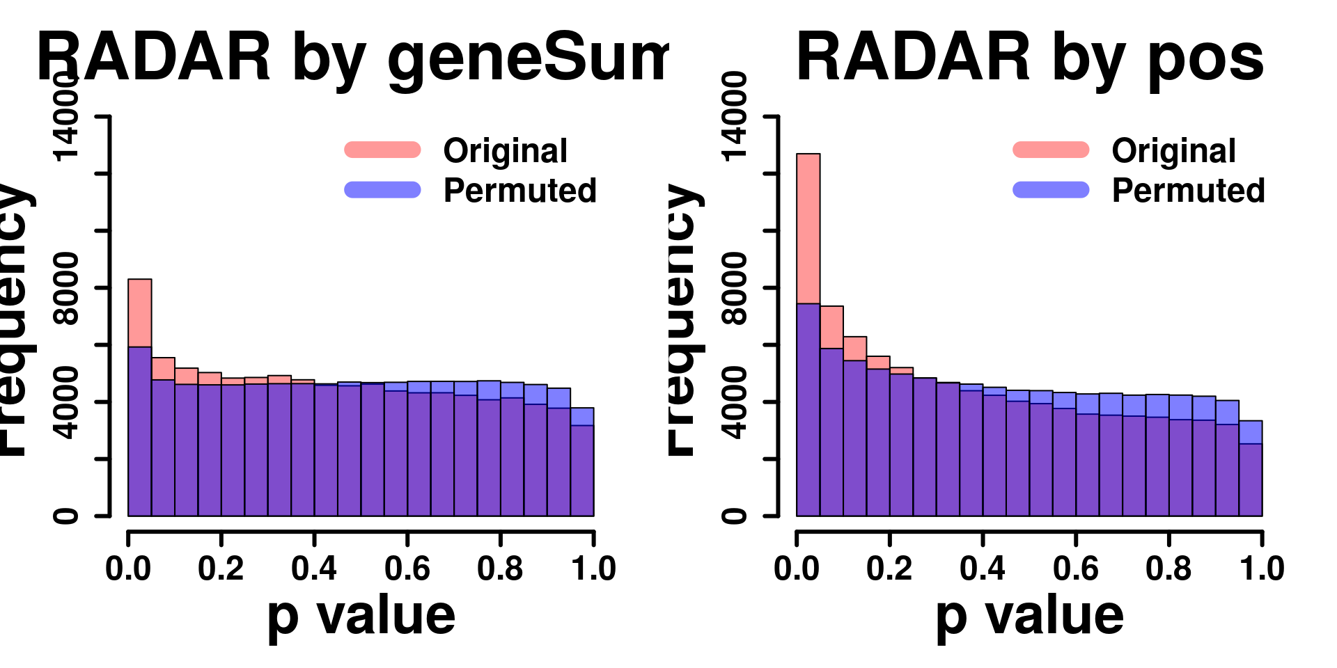

Report differential peaks

RADAR <- reportResult(RADAR, cutoff = 0.1,threads = 20)
Diff_peaks <- results(RADAR)

reportPeaks <- function(radar, est , cutoff = 0.1, Beta_cutoff = 0.5, threads = 1){
  stats <- est
  rownames(stats) <- rownames(radar@test.est)
  colnames(stats) <- gsub("padj","fdr",colnames(stats))
  colnames(stats) <- gsub("log2.OR","beta",colnames(stats))
  colnames(stats) <- gsub("logFC","beta",colnames(stats))
  colnames(stats) <- gsub("log2.OR","beta",colnames(stats))
  colnames(stats) <- gsub("pvalue","p_value",colnames(stats))
   
  num_bins <- length( which(stats[,"fdr"] < cutoff & abs(stats[,"beta"] )> Beta_cutoff) )
  if(num_bins < 1 ){
    stop("There is no bin passing the threshold...\n No differential peaks can be reported at current cutoff...")
  }else {
    sig.bins <- rownames(stats)[which(stats[,"fdr"] < cutoff & abs(stats[,"beta"] )> Beta_cutoff)]
  }
  
  geneBins <- geneBins(radar)
  ID <- (rownames(geneBins) %in% sig.bins)
  
  num_lines <- length(ID)
  
  # start ids of checkpoints
  ## find peak-starting checkpoints (either from nonpeak to peak, or peak in a different batch)
  start_id <- which((ID[2:num_lines]-ID[1:num_lines-1]==1) |
                      ((geneBins$gene[2:num_lines]!=geneBins$gene[1:num_lines-1]) & (ID[2:num_lines] == TRUE)) )
  start_id <- start_id + 1 # add 1 since ID was counted from 2 to num_lines
  if ( ID[1]==TRUE ) { start_id <- c(1,start_id) } # if the first checkpoint bin is peak
  
  # end ids of checkpoints
  ## find peak-ending checkpoints (either from peak to nonpeak, or peak in a different batch)
  end_id <- which((ID[1:num_lines-1]-ID[2:num_lines]==1) |
                    ((geneBins$gene[1:num_lines-1]!=geneBins$gene[2:num_lines]) & (ID[1:num_lines-1] == TRUE)) )
  if (ID[num_lines]==TRUE) {end_id <- c(end_id,num_lines)} # if the last checkpoint bin is peak
  
  peak_id_pairs <- cbind(start_id, end_id)
  num_peaks <- nrow(peak_id_pairs)
  geneGRList <- radar@geneModel
  peakGenes <- as.character(geneBins[peak_id_pairs[,1],"gene"])
  
  cat(paste0("reporting ",num_peaks," of peaks\n"))
  if (num_peaks == 0){return(data.frame())
  }else{
    start_time <- Sys.time()
    registerDoParallel(cores = threads)
    cat(paste("Hyper-thread registered:",getDoParRegistered(),"\n"))
    cat(paste("Using",getDoParWorkers(),"thread(s) to report merged report...\n"))
    merged.report<- foreach( p = 1:num_peaks, .combine = rbind)%dopar%{
      peak_row_id <- peak_id_pairs[p,]
      geneExons <- reduce ( geneGRList[peakGenes[p]][[1]] )
      
      peak <- RADAR:::.getPeakBins(geneGRList,peakGenes[p],c(geneBins$bin[peak_row_id[1]],geneBins$bin[peak_row_id[2]]),radar@binSize )
      
      peakE <- RADAR:::.peakExons(peak,as.data.frame(geneExons))
      data.frame(chr=peak$chr,
                 start = peak$start,
                 end = peak$end,
                 name = peakGenes[p],
                 score = 0,
                 strand = as.character(strand(geneExons))[1],
                 thickStart = peak$start,
                 thickEnd = peak$end,
                 itemRgb=0,
                 blockCount = nrow(peakE),
                 blockSizes = paste(peakE$width,collapse=","),
                 blockStarts = paste(peakE$start - replicate(nrow(peakE),peakE$start[1]),collapse=","),
                 logFC = stats[rownames(geneBins[peak_row_id[1]:peak_row_id[2],]), "beta"][which.max(abs( stats[rownames(geneBins[peak_row_id[1]:peak_row_id[2],]), "beta"] ))],
                 p_value = RADAR:::.fishersMethod(  stats[rownames(geneBins[peak_row_id[1]:peak_row_id[2],]), "p_value"] )
      )
    }
    rm(list=ls(name=foreach:::.foreachGlobals), pos=foreach:::.foreachGlobals)
    end_time <- Sys.time()
    cat(paste("Time used to report peaks:",difftime(end_time, start_time, units = "mins"),"mins... \n"))
  }
  
  return(merged.report)
  
}

exomePeak_diff <- reportPeaks(RADAR, est = exomePeak.res, threads = 20)
QNB_diff <- reportPeaks(RADAR, est = QNB.res, threads = 20)
Metdiff_diff <- reportPeaks(RADAR, est = Metdiff.res, threads = 20)
fisher_diff <- reportPeaks(RADAR, est = fisher.res, threads = 20)

library(MeRIPtools)
plotMetaGeneMulti(list("RADAR" = Diff_peaks,"exomePeak"=exomePeak_diff, "QNB" = QNB_diff, "MeTDiff" = Metdiff_diff, "Fisher" = fisher_diff ),"~/Database/genome/mm10/mm10_UCSC.gtf")

## [1] "Converting BED12 to GRangesList"
## [1] "It may take a few minutes"
## [1] "Converting BED12 to GRangesList"
## [1] "It may take a few minutes"
## [1] "Converting BED12 to GRangesList"
## [1] "It may take a few minutes"
## [1] "Converting BED12 to GRangesList"
## [1] "It may take a few minutes"
## [1] "Converting BED12 to GRangesList"
## [1] "It may take a few minutes"
## [1] "total 35119 transcripts extracted ..."
## [1] "total 31408 transcripts left after ambiguity filter ..."
## [1] "total 15627 mRNAs left after component length filter ..."
## [1] "total 3280 ncRNAs left after ncRNA length filter ..."
## [1] "Building Guitar Coordinates. It may take a few minutes ..."
## [1] "Guitar Coordinates Built ..."
## [1] "Using provided Guitar Coordinates"
## [1] "resolving ambiguious features ..."
## [1] "no figure saved ..."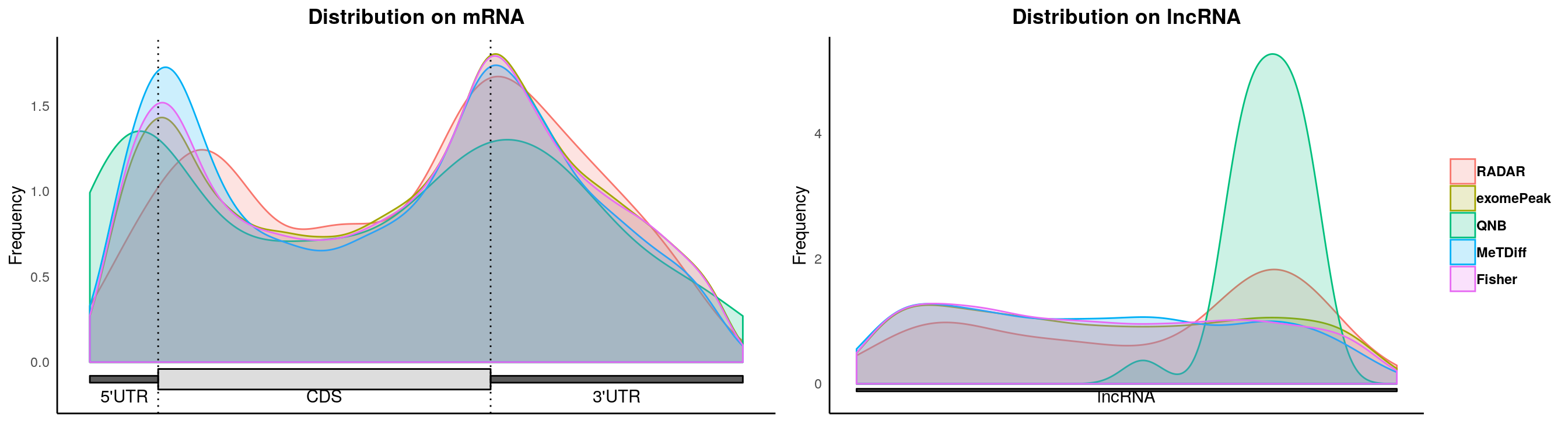

## NOTE this function is a wrapper for R package "Guitar".
## If you use the metaGene plot in publication, please cite the original reference:
## Cui et al 2016 BioMed Research International

plotMetaGeneMulti(list("RADAR" = Diff_peaks,"exomePeak"=exomePeak_diff,  "MeTDiff" = Metdiff_diff, "Fisher" = fisher_diff ),"~/Database/genome/mm10/mm10_UCSC.gtf")

## [1] "Converting BED12 to GRangesList"
## [1] "It may take a few minutes"
## [1] "Converting BED12 to GRangesList"
## [1] "It may take a few minutes"
## [1] "Converting BED12 to GRangesList"
## [1] "It may take a few minutes"
## [1] "Converting BED12 to GRangesList"
## [1] "It may take a few minutes"
## [1] "total 35119 transcripts extracted ..."
## [1] "total 31408 transcripts left after ambiguity filter ..."
## [1] "total 15627 mRNAs left after component length filter ..."
## [1] "total 3280 ncRNAs left after ncRNA length filter ..."
## [1] "Building Guitar Coordinates. It may take a few minutes ..."
## [1] "Guitar Coordinates Built ..."
## [1] "Using provided Guitar Coordinates"
## [1] "resolving ambiguious features ..."
## [1] "no figure saved ..."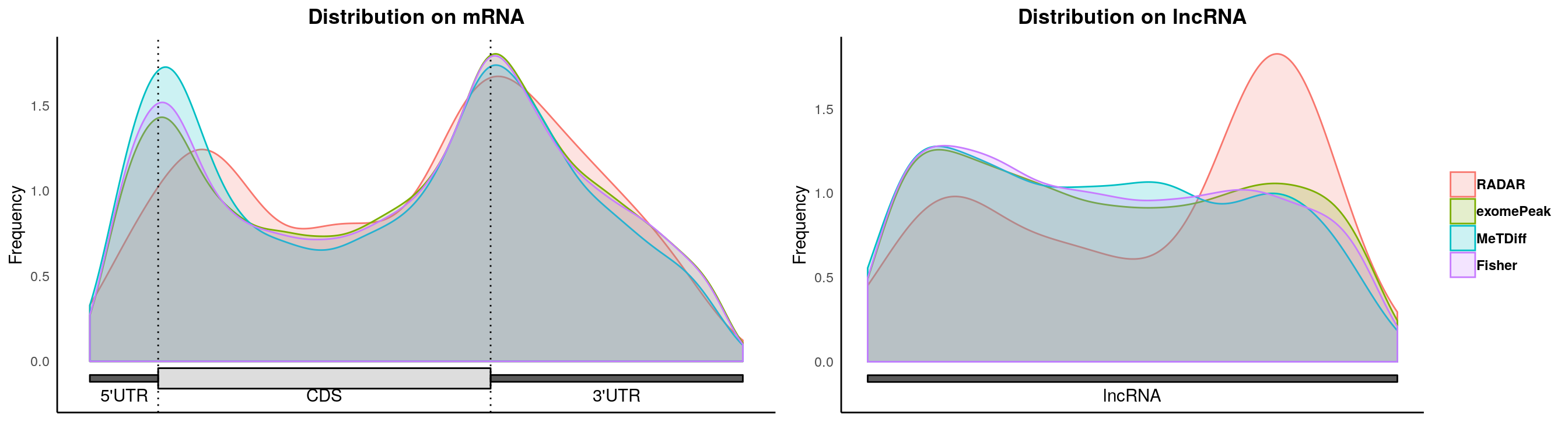

## NOTE this function is a wrapper for R package "Guitar".
## If you use the metaGene plot in publication, please cite the original reference:
## Cui et al 2016 BioMed Research International

detach("package:MeRIPtools", unload = TRUE)

extendPeak <- function(peak, extension = 50){
  peak_extend <- peak
  peak_extend$start <- peak$start-extension
  peak_extend$end <- peak$end+extension
  
  peak_extend$blockSizes <- unlist( lapply( strsplit(as.character(peak$blockSizes),split = ",") , function(x){
    tmp = as.numeric(x)
    tmp[1] = tmp[1]+extension
    tmp[length(tmp)] = tmp[length(tmp)]+extension
    paste(as.character(tmp),collapse  = ",")
    }  ) )
  return(peak_extend)
}

Diff_peaks_extend <- extendPeak(Diff_peaks)

exomePeak_diff_extend <- extendPeak(exomePeak_diff)
Metdiff_diff_extend <- extendPeak(Metdiff_diff)

## analysis for RADAR detected signifiant bins
write.table(Diff_peaks_extend[,1:12], file = paste0("~/Tools/RADARmannual/data/mouseLiver_Diff_peaks_ageCov.bed"),sep = "\t",row.names = F,col.names = F,quote = F)
system2(command = "bedtools", args = paste0("getfasta -fi ~/Database/genome/mm10/mm10_UCSC.fa -bed ~/Tools/RADARmannual/data/mouseLiver_Diff_peaks_ageCov.bed -s -split > ~/Tools/RADARmannual/data/mouseLiver_Diff_peaks_ageCov.fa ") )

system2(command = "findMotifs.pl", args = paste0("~/Tools/RADARmannual/data/mouseLiver_Diff_peaks_ageCov.fa fasta ~/Tools/RADARmannual/data/mouseLiver_Diff_peaks_ageCov_Homer2 -fasta ~/Database/transcriptome/backgroud_peaks/mm10_80bpRandomPeak.fa -len 5,6 -rna -p 20 -S 5 -noknown"),wait = F )

## analysis for exomePeak detected significant bins
write.table(exomePeak_diff_extend[,1:12], file = paste0("~/Tools/RADARmannual/data/mouseLiver_Diff_exomePeak.bed"),sep = "\t",row.names = F,col.names = F,quote = F)
system2(command = "bedtools", args = paste0("getfasta -fi ~/Database/genome/mm10/mm10_UCSC.fa -bed ~/Tools/RADARmannual/data/mouseLiver_Diff_exomePeak.bed -s -split > ~/Tools/RADARmannual/data/mouseLiver_Diff_exomePeak.fa ") )

system2(command = "findMotifs.pl", args = paste0("~/Tools/RADARmannual/data/mouseLiver_Diff_exomePeak.fa fasta ~/Tools/RADARmannual/data/mouseLiver_Diff_exomePeak_Homer2 -fasta ~/Database/transcriptome/backgroud_peaks/mm10_80bpRandomPeak.fa -len 5,6 -rna -p 20 -S 5 -noknown"),wait = F )

## analysis for MetDiff detected significant bins
write.table(Metdiff_diff_extend[,1:12], file = paste0("~/Tools/RADARmannual/data/mouseLiver_Diff_MetDiff.bed"),sep = "\t",row.names = F,col.names = F,quote = F)
system2(command = "bedtools", args = paste0("getfasta -fi ~/Database/genome/mm10/mm10_UCSC.fa -bed ~/Tools/RADARmannual/data/mouseLiver_Diff_MetDiff.bed -s -split > ~/Tools/RADARmannual/data/mouseLiver_Diff_MetDiff.fa ") )

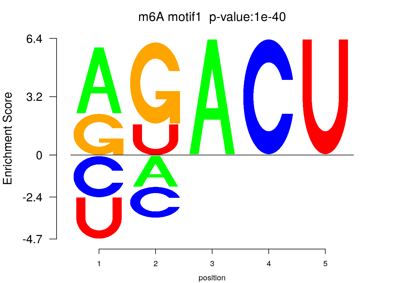
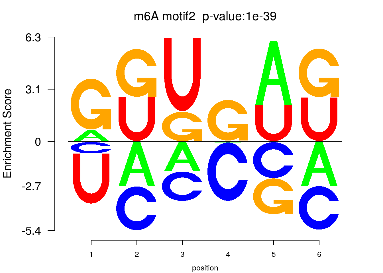
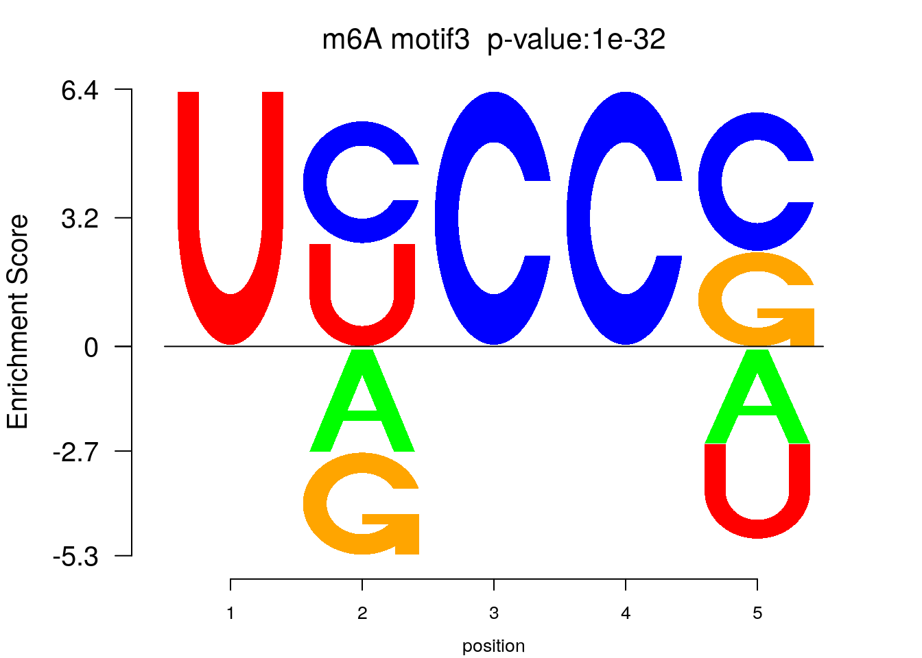
system2(command = "findMotifs.pl", args = paste0("~/Tools/RADARmannual/data/mouseLiver_Diff_MetDiff.fa fasta ~/Tools/RADARmannual/data/mouseLiver_Diff_MetDiff_Homer2 -fasta ~/Database/transcriptome/backgroud_peaks/mm10_80bpRandomPeak.fa -len 5,6 -rna -p 20 -S 5 -noknown"),wait = F )

library(Logolas)
color_motif <- c( "orange", "blue", "red","green" )
for(i in 1:3){
  pwm.m <- t( read.table(paste0("~/Tools/RADARmannual/data/mouseLiver_Diff_peaks_ageCov_Homer2/homerResults/motif",i,".motif"), header = F, comment.char = ">",col.names = c("A","C","G","U")) )
  motif_p <- sapply(1:3, function(x){
   strsplit( as.character( read.table(paste0("~/Tools/RADARmannual/data/mouseLiver_Diff_peaks_ageCov_Homer2/homerResults/motif",x,".motif"),comment.char = "", nrows = 1)[,12]  ), split= ":")[[1]][4] 
})
  colnames(pwm.m) <- 1:ncol(pwm.m)

  try(logomaker(pwm.m ,type = "EDLogo",colors = color_motif,color_type = "per_row" ,logo_control =  list(pop_name = paste0("m6A motif",i,"  p-value:",motif_p[i])))
  )

}

Session information

sessionInfo()

## R version 3.5.3 (2019-03-11)
## Platform: x86_64-pc-linux-gnu (64-bit)
## Running under: Ubuntu 17.10
## 
## Matrix products: default
## BLAS: /usr/lib/x86_64-linux-gnu/openblas/libblas.so.3
## LAPACK: /usr/lib/x86_64-linux-gnu/libopenblasp-r0.2.20.so
## 
## locale:
##  [1] LC_CTYPE=en_US.UTF-8       LC_NUMERIC=C              
##  [3] LC_TIME=en_US.UTF-8        LC_COLLATE=en_US.UTF-8    
##  [5] LC_MONETARY=en_US.UTF-8    LC_MESSAGES=en_US.UTF-8   
##  [7] LC_PAPER=en_US.UTF-8       LC_NAME=C                 
##  [9] LC_ADDRESS=C               LC_TELEPHONE=C            
## [11] LC_MEASUREMENT=en_US.UTF-8 LC_IDENTIFICATION=C       
## 
## attached base packages:
##  [1] grid      stats4    parallel  stats     graphics  grDevices utils    
##  [8] datasets  methods   base     
## 
## other attached packages:
##  [1] Logolas_1.6.0               reshape2_1.4.3             
##  [3] GenomicAlignments_1.18.1    SummarizedExperiment_1.12.0
##  [5] DelayedArray_0.8.0          BiocParallel_1.16.6        
##  [7] matrixStats_0.54.0          rtracklayer_1.42.2         
##  [9] RADAR_0.2.1                 qvalue_2.14.1              
## [11] RcppArmadillo_0.9.400.2.0   Rcpp_1.0.1                 
## [13] RColorBrewer_1.1-2          gplots_3.0.1.1             
## [15] doParallel_1.0.14           iterators_1.0.10           
## [17] foreach_1.4.4               ggplot2_3.1.1              
## [19] Rsamtools_1.34.1            Biostrings_2.50.2          
## [21] XVector_0.22.0              GenomicFeatures_1.34.8     
## [23] AnnotationDbi_1.44.0        Biobase_2.42.0             
## [25] GenomicRanges_1.34.0        GenomeInfoDb_1.18.2        
## [27] IRanges_2.16.0              S4Vectors_0.20.1           
## [29] BiocGenerics_0.28.0        
## 
## loaded via a namespace (and not attached):
##   [1] backports_1.1.4        Hmisc_4.2-0            fastmatch_1.1-0       
##   [4] plyr_1.8.4             igraph_1.2.4.1         lazyeval_0.2.2        
##   [7] splines_3.5.3          gamlss_5.1-3           gridBase_0.4-7        
##  [10] urltools_1.7.3         digest_0.6.18          htmltools_0.3.6       
##  [13] GOSemSim_2.8.0         viridis_0.5.1          GO.db_3.7.0           
##  [16] SQUAREM_2017.10-1      gdata_2.18.0           magrittr_1.5          
##  [19] checkmate_1.9.1        memoise_1.1.0          BSgenome_1.50.0       
##  [22] cluster_2.0.7-1        annotate_1.60.1        enrichplot_1.2.0      
##  [25] prettyunits_1.0.2      colorspace_1.4-1       blob_1.1.1            
##  [28] ggrepel_0.8.0          gamlss.data_5.1-3      exomePeak_2.16.0      
##  [31] xfun_0.6               dplyr_0.8.0.1          crayon_1.3.4          
##  [34] RCurl_1.95-4.12        jsonlite_1.6           genefilter_1.64.0     
##  [37] ape_5.3                survival_2.44-1.1      glue_1.3.1            
##  [40] polyclip_1.10-0        gtable_0.3.0           zlibbioc_1.28.0       
##  [43] UpSetR_1.3.3           scales_1.0.0           DOSE_3.8.2            
##  [46] DBI_1.0.0              viridisLite_0.3.0      xtable_1.8-4          
##  [49] progress_1.2.0         htmlTable_1.13.1       gridGraphics_0.3-0    
##  [52] foreign_0.8-71         bit_1.1-14             europepmc_0.3         
##  [55] Formula_1.2-3          htmlwidgets_1.3        httr_1.4.0            
##  [58] fgsea_1.8.0            acepack_1.4.1          pkgconfig_2.0.2       
##  [61] XML_3.98-1.19          farver_1.1.0           nnet_7.3-12           
##  [64] locfit_1.5-9.1         ggplotify_0.0.3        tidyselect_0.2.5      
##  [67] labeling_0.3           rlang_0.4.0            munsell_0.5.0         
##  [70] tools_3.5.3            generics_0.0.2         RSQLite_2.1.1         
##  [73] broom_0.5.2            ggridges_0.5.1         evaluate_0.13         
##  [76] stringr_1.4.0          yaml_2.2.0             knitr_1.22            
##  [79] bit64_0.9-7            fs_1.3.0               caTools_1.17.1.2      
##  [82] purrr_0.3.2            ggraph_1.0.2           nlme_3.1-137          
##  [85] QNB_1.1.11             DO.db_2.9              xml2_1.2.0            
##  [88] biomaRt_2.38.0         compiler_3.5.3         rstudioapi_0.10       
##  [91] Guitar_1.20.1          tibble_2.1.1           tweenr_1.0.1          
##  [94] geneplotter_1.60.0     stringi_1.4.3          lattice_0.20-38       
##  [97] Matrix_1.2-17          permute_0.9-5          vegan_2.5-4           
## [100] pillar_1.3.1           triebeard_0.3.0        data.table_1.12.2     
## [103] cowplot_0.9.4          bitops_1.0-6           R6_2.4.0              
## [106] latticeExtra_0.6-28    vcfR_1.8.0             KernSmooth_2.23-15    
## [109] gridExtra_2.3          codetools_0.2-16       MASS_7.3-51.4         
## [112] gtools_3.8.1           assertthat_0.2.1       DESeq2_1.22.2         
## [115] pinfsc50_1.1.0         withr_2.1.2            GenomeInfoDbData_1.2.0
## [118] mgcv_1.8-28            hms_0.4.2              clusterProfiler_3.10.1
## [121] rpart_4.1-13           tidyr_0.8.3            rmarkdown_1.12        
## [124] rvcheck_0.1.3          ggforce_0.2.2          gamlss.dist_5.1-3     
## [127] base64enc_0.1-3

This R Markdown site was created with workflowr