Analyzing MeRIP-seq data with RADAR
Zijie Zhang, Chuan He, Mengjie Chen
26 November 2018
Abstract
A basic task in the analysis of MeRIP-seq is the detection of differentially methylated loci on the RNA. To analyze the count data of MeRIP-seq, we divide the transcript (concatenated exons of a gene) into consecutive bins and quantify the reads align to each bin. The summarized count data is in matrix format where each row represent a locus and each column is a sample. Statistical inference of changes across group, as compared to within-group variability was made for each filtered bin with sufficient count. This vignette explains the use of the package RADAR with example data. RADAR package version: 0.1.5
Note: if you use RADAR in published research, please cite:
Other Bioconductor packages with similar aims are exomePeak, MeTDiff, QNB.
1.Quick start
Here we show the most basic steps for a differential methylation analysis. There is one major steps upstream of radar that generate mapped reads in BAM files for each sample, which can be done by varies choices of softwares such as Hisat2, tophat2 or Kallisto. we will discuss in the sections below assuming BAM file has been obtained.
This code chunk assumes that you have bam files for sample1-6 s1.input.bam... s6..input.bam and s1.m6A.bam... s6..m6A.bam and a vector of group asignment X = c("Ctl","Ctl","Ctl","Treated","Treated","Treated").
library(RADAR)
radar <- countReads(
  samplenames = c("s1","s2","s3","s4","s5","s6"),
  gtf = "/path/to/file.gtf",
  bamFolder = "/path/to/bam files",
  modification = "m6A",
  strandToKeep = "opposite"
)

radar <- normalizeLibrary( radar, X )
radar <- adjustExprLevel( radar )
radar <- filterBins( radar ,minCountsCutOff = 15)
radar <- diffIP(radar)
## if using linux or mac, you can also use multi-thread mode
radar <- diffIP_parallel(radar)
res <- reportPoissonGammaMerge(radar,cutoff = 0.1)
2.How to get help for
Issues and questions about the package should be posted to the issue report page of the github. The issue discussed here can served as public knowledge base.
3.Standard workflow
a). Mapped BAM file.
To analyze for MeRIP-seq data, RADAR expect a pair of BAM file for each sample. For each pair of BAM file, the naming convention for RADAR is sample.input.bam for INPUT and sample.m6A.bam for m6A IP or sample.m1A.bam for m1A IP sample. They key is INPUT and IP sample have the same prefix.
b). GTF annotation file.
For the organism being analyzed, user need to provide an annotation file in gtf format to define the genomic coordinate of gene features. A good source to download those supporting files are iGenome.
c). The RADAR DataSet
The List object used by the RADAR package to store the read counts and associated parameters, which will usually be represented in the code here as an object radar.
We will use a toy data set to demonstrate how to start from bam file to count reads in consecutive bins and construct a RADAR dataset. There are 9 contols and 8 cases sample in the toy dataset. We name them by Ctl# and Case# in the follow demonstrations.
Please note that user should set bam_dir to directory where bam files are saved instead of setting it to package assocated example file folder system.file("extdata",package = "RADAR").
library(RADAR)
samplenames <- c( paste0("Ctl",1:9), paste0("Case",1:8) )
bam_dir <- system.file('extdata',package = 'RADAR')
samplenames
## [1] "Ctl1" "Ctl2" "Ctl3" "Ctl4" "Ctl5" "Ctl6" "Ctl7" "Ctl8"
## [9] "Ctl9" "Case1" "Case2" "Case3" "Case4" "Case5" "Case6" "Case7"
## [17] "Case8"Here we created a character vector samplenames to define the names of sample, which will later tells RADAR to look for input and IP file with prefix samplenames.
Next we need to use countReads() function to 1) concatenate exons of each gene to get a “longest isoform” transcript of each gene. 2) Divide transcripts into consecutive bins of user defined width. 3) count reads mapped to each bin.
note1 The parameter modification = "m6A" tells the function to look for bam file of IP by the name samplename.m6A.bam. If the user named the IP sample as samplename.IP.bam, modification should be set to modification = "IP. We enable flexible seeting for IP sample in cases where user perform MeRIP seq on multiple modification with shared INPUT library.
note2 In Linux or MacOs, our package support multi-thread mode enabled by R package doParallel . One can set the number of threads to use by threads = n.
note3 The default setting for bin width to slice the transcript is 50bp. One can set this by parameter binSize = #bp. For very shallow sequencing depth (e.g. less than 10M mappable reads per library), we recommand setting bin width to larger size such as 100bp to increase the number of reads countable in each bin.
note4 The parameter fragmentLength defines the number of nucleotide to shift from the head of a read in BAM record to the center of RNA fragment. In the example data, the RNA has been sonicated into ~150nt fragment before IP and library preparation.
radar <- countReads(samplenames = samplenames,
                    gtf = "~/Database/genome/hg38/hg38_UCSC.gtf",
                    bamFolder = bam_dir,
                    modification = "m6A",
                    fragmentLength = 150,
                    outputDir = "test",
                    threads = 20,
                    binSize = 50
)
## [1] "Stage: index bam file /home/zijiezhang/R/x86_64-pc-linux-gnu-library/3.5/RADAR/extdata/Ctl1.input.bam"
## [1] "Stage: index bam file /home/zijiezhang/R/x86_64-pc-linux-gnu-library/3.5/RADAR/extdata/Ctl1.m6A.bam"
## [1] "Stage: index bam file /home/zijiezhang/R/x86_64-pc-linux-gnu-library/3.5/RADAR/extdata/Ctl2.input.bam"
## [1] "Stage: index bam file /home/zijiezhang/R/x86_64-pc-linux-gnu-library/3.5/RADAR/extdata/Ctl2.m6A.bam"
## [1] "Stage: index bam file /home/zijiezhang/R/x86_64-pc-linux-gnu-library/3.5/RADAR/extdata/Ctl3.input.bam"
## [1] "Stage: index bam file /home/zijiezhang/R/x86_64-pc-linux-gnu-library/3.5/RADAR/extdata/Ctl3.m6A.bam"
## [1] "Stage: index bam file /home/zijiezhang/R/x86_64-pc-linux-gnu-library/3.5/RADAR/extdata/Ctl4.input.bam"
## [1] "Stage: index bam file /home/zijiezhang/R/x86_64-pc-linux-gnu-library/3.5/RADAR/extdata/Ctl4.m6A.bam"
## [1] "Stage: index bam file /home/zijiezhang/R/x86_64-pc-linux-gnu-library/3.5/RADAR/extdata/Ctl5.input.bam"
## [1] "Stage: index bam file /home/zijiezhang/R/x86_64-pc-linux-gnu-library/3.5/RADAR/extdata/Ctl5.m6A.bam"
## [1] "Stage: index bam file /home/zijiezhang/R/x86_64-pc-linux-gnu-library/3.5/RADAR/extdata/Ctl6.input.bam"
## [1] "Stage: index bam file /home/zijiezhang/R/x86_64-pc-linux-gnu-library/3.5/RADAR/extdata/Ctl6.m6A.bam"
## [1] "Stage: index bam file /home/zijiezhang/R/x86_64-pc-linux-gnu-library/3.5/RADAR/extdata/Ctl7.input.bam"
## [1] "Stage: index bam file /home/zijiezhang/R/x86_64-pc-linux-gnu-library/3.5/RADAR/extdata/Ctl7.m6A.bam"
## [1] "Stage: index bam file /home/zijiezhang/R/x86_64-pc-linux-gnu-library/3.5/RADAR/extdata/Ctl8.input.bam"
## [1] "Stage: index bam file /home/zijiezhang/R/x86_64-pc-linux-gnu-library/3.5/RADAR/extdata/Ctl8.m6A.bam"
## [1] "Stage: index bam file /home/zijiezhang/R/x86_64-pc-linux-gnu-library/3.5/RADAR/extdata/Ctl9.input.bam"
## [1] "Stage: index bam file /home/zijiezhang/R/x86_64-pc-linux-gnu-library/3.5/RADAR/extdata/Ctl9.m6A.bam"
## [1] "Stage: index bam file /home/zijiezhang/R/x86_64-pc-linux-gnu-library/3.5/RADAR/extdata/Case1.input.bam"
## [1] "Stage: index bam file /home/zijiezhang/R/x86_64-pc-linux-gnu-library/3.5/RADAR/extdata/Case1.m6A.bam"
## [1] "Stage: index bam file /home/zijiezhang/R/x86_64-pc-linux-gnu-library/3.5/RADAR/extdata/Case2.input.bam"
## [1] "Stage: index bam file /home/zijiezhang/R/x86_64-pc-linux-gnu-library/3.5/RADAR/extdata/Case2.m6A.bam"
## [1] "Stage: index bam file /home/zijiezhang/R/x86_64-pc-linux-gnu-library/3.5/RADAR/extdata/Case3.input.bam"
## [1] "Stage: index bam file /home/zijiezhang/R/x86_64-pc-linux-gnu-library/3.5/RADAR/extdata/Case3.m6A.bam"
## [1] "Stage: index bam file /home/zijiezhang/R/x86_64-pc-linux-gnu-library/3.5/RADAR/extdata/Case4.input.bam"
## [1] "Stage: index bam file /home/zijiezhang/R/x86_64-pc-linux-gnu-library/3.5/RADAR/extdata/Case4.m6A.bam"
## [1] "Stage: index bam file /home/zijiezhang/R/x86_64-pc-linux-gnu-library/3.5/RADAR/extdata/Case5.input.bam"
## [1] "Stage: index bam file /home/zijiezhang/R/x86_64-pc-linux-gnu-library/3.5/RADAR/extdata/Case5.m6A.bam"
## [1] "Stage: index bam file /home/zijiezhang/R/x86_64-pc-linux-gnu-library/3.5/RADAR/extdata/Case6.input.bam"
## [1] "Stage: index bam file /home/zijiezhang/R/x86_64-pc-linux-gnu-library/3.5/RADAR/extdata/Case6.m6A.bam"
## [1] "Stage: index bam file /home/zijiezhang/R/x86_64-pc-linux-gnu-library/3.5/RADAR/extdata/Case7.input.bam"
## [1] "Stage: index bam file /home/zijiezhang/R/x86_64-pc-linux-gnu-library/3.5/RADAR/extdata/Case7.m6A.bam"
## [1] "Stage: index bam file /home/zijiezhang/R/x86_64-pc-linux-gnu-library/3.5/RADAR/extdata/Case8.input.bam"
## [1] "Stage: index bam file /home/zijiezhang/R/x86_64-pc-linux-gnu-library/3.5/RADAR/extdata/Case8.m6A.bam"
## Reading gtf file to obtain gene model
## Filter out ambiguous model...
## Gene model obtained from gtf file...
## counting reads for each genes, this step may takes a few hours....
## Hyper-thread registered: TRUE
## Using 20 thread(s) to count reads in continuous bins...
## Time used to count reads: 18.4296131491661 mins...Now we have read count of consecutive 50bp bins for each sample. The count data is saved as a matrix object in the return List object radar. The count matrix can be returned by radar$reads. We can take a look at the content of the radar object.
lapply(radar,head)## $reads
## Ctl1-input Ctl2-input Ctl3-input Ctl4-input Ctl5-input Ctl6-input
## A1BG,25 0 0 0 0 0 0
## A1BG,74 0 0 0 0 0 0
## A1BG,123 0 0 0 0 0 0
## A1BG,172 0 0 0 0 0 0
## A1BG,221 0 0 0 0 0 0
## A1BG,270 0 0 0 0 0 0
## Ctl7-input Ctl8-input Ctl9-input Case1-input Case2-input
## A1BG,25 0 0 0 0 0
## A1BG,74 0 0 0 0 0
## A1BG,123 0 0 0 0 0
## A1BG,172 0 0 0 0 0
## A1BG,221 0 0 0 0 0
## A1BG,270 0 0 0 0 0
## Case3-input Case4-input Case5-input Case6-input Case7-input
## A1BG,25 0 0 0 0 0
## A1BG,74 0 0 0 0 0
## A1BG,123 0 0 0 0 0
## A1BG,172 0 0 0 0 0
## A1BG,221 0 0 0 0 0
## A1BG,270 0 0 0 0 0
## Case8-input Ctl1-IP Ctl2-IP Ctl3-IP Ctl4-IP Ctl5-IP Ctl6-IP
## A1BG,25 0 0 0 0 0 0 0
## A1BG,74 0 0 0 0 0 0 0
## A1BG,123 0 0 0 0 0 0 0
## A1BG,172 0 0 0 0 0 0 0
## A1BG,221 0 0 0 0 0 0 0
## A1BG,270 0 0 0 0 0 0 0
## Ctl7-IP Ctl8-IP Ctl9-IP Case1-IP Case2-IP Case3-IP Case4-IP
## A1BG,25 0 0 0 0 0 0 0
## A1BG,74 0 0 0 0 0 0 0
## A1BG,123 0 0 0 0 0 0 0
## A1BG,172 0 0 0 0 0 0 0
## A1BG,221 0 0 0 0 0 0 0
## A1BG,270 0 0 0 0 0 0 0
## Case5-IP Case6-IP Case7-IP Case8-IP
## A1BG,25 0 0 0 0
## A1BG,74 0 0 0 0
## A1BG,123 0 0 0 0
## A1BG,172 0 0 0 0
## A1BG,221 0 0 0 0
## A1BG,270 0 0 0 0
##
## $binSize
## [1] 50
##
## $geneModel
## GRangesList object of length 6:
## $A1BG
## GRanges object with 8 ranges and 2 metadata columns:
## seqnames ranges strand | exon_id exon_name
## <Rle> <IRanges> <Rle> | <integer> <character>
## [1] chr19 58346806-58347029 - | 220303 <NA>
## [2] chr19 58347353-58347640 - | 220304 <NA>
## [3] chr19 58350370-58350651 - | 220305 <NA>
## [4] chr19 58351391-58351687 - | 220306 <NA>
## [5] chr19 58352283-58352555 - | 220307 <NA>
## [6] chr19 58352928-58353197 - | 220308 <NA>
## [7] chr19 58353292-58353327 - | 220309 <NA>
## [8] chr19 58353404-58353499 - | 220310 <NA>
##
## $A1BG-AS1
## GRanges object with 4 ranges and 2 metadata columns:
## seqnames ranges strand | exon_id exon_name
## [1] chr19 58351970-58353044 + | 213488 <NA>
## [2] chr19 58353379-58353474 + | 213489 <NA>
## [3] chr19 58353714-58353857 + | 213490 <NA>
## [4] chr19 58354369-58355183 + | 213491 <NA>
##
## ...
## <4 more elements>
## -------
## seqinfo: 24 sequences from an unspecified genome; no seqlengths
##
## $bamPath.input
## [1] "/home/zijiezhang/R/x86_64-pc-linux-gnu-library/3.5/RADAR/extdata/Ctl1.input.bam"
## [2] "/home/zijiezhang/R/x86_64-pc-linux-gnu-library/3.5/RADAR/extdata/Ctl2.input.bam"
## [3] "/home/zijiezhang/R/x86_64-pc-linux-gnu-library/3.5/RADAR/extdata/Ctl3.input.bam"
## [4] "/home/zijiezhang/R/x86_64-pc-linux-gnu-library/3.5/RADAR/extdata/Ctl4.input.bam"
## [5] "/home/zijiezhang/R/x86_64-pc-linux-gnu-library/3.5/RADAR/extdata/Ctl5.input.bam"
## [6] "/home/zijiezhang/R/x86_64-pc-linux-gnu-library/3.5/RADAR/extdata/Ctl6.input.bam"
##
## $bamPath.ip
## [1] "/home/zijiezhang/R/x86_64-pc-linux-gnu-library/3.5/RADAR/extdata/Ctl1.m6A.bam"
## [2] "/home/zijiezhang/R/x86_64-pc-linux-gnu-library/3.5/RADAR/extdata/Ctl2.m6A.bam"
## [3] "/home/zijiezhang/R/x86_64-pc-linux-gnu-library/3.5/RADAR/extdata/Ctl3.m6A.bam"
## [4] "/home/zijiezhang/R/x86_64-pc-linux-gnu-library/3.5/RADAR/extdata/Ctl4.m6A.bam"
## [5] "/home/zijiezhang/R/x86_64-pc-linux-gnu-library/3.5/RADAR/extdata/Ctl5.m6A.bam"
## [6] "/home/zijiezhang/R/x86_64-pc-linux-gnu-library/3.5/RADAR/extdata/Ctl6.m6A.bam"
##
## $samplenames
## [1] "Ctl1" "Ctl2" "Ctl3" "Ctl4" "Ctl5" "Ctl6"As shown, we can see countReads() function returns a List object of 6 elements. RMD$reads stores the read count matrix. radar$binSize stores the width of the bin to slice the transcript. radar$geneModel is a genomic range list object store the exons of each gene.
e). Normalization and Filtering
After obtaining the radar object containing read count, we can then proceed to library normalization step. This step requires the user to define the grouping infomation by a vector parameter X.
X <- c(rep("Ctl",9),rep("Case",8))
plot.new()
radar <- normalizeLibrary(radar,X)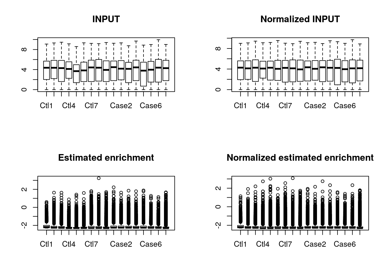
In this step, the bin-level read count of input is summarized into gene-level read count. The size factor of input is calculated using “mean ratio method” implemented in DESeq2, which is then used to calculated normalized input bin-level read count. To normalize the library size of IP samples, we use top-read-count bins of IP and corresponding input gene-level read count to compute the enrichment esimate of each sample. Under the assumption that samples in the same study have same IP efficiency, we normalize the IP by normalizing the estimated IP efficiency. As an sanity check, in addition to return the radar object with normalized read count, the normalizeLibrary() function also generate box plot of read count before and after normalizing INPUT and box plot of estimated enrichment before and after normalizing IP.
In the returned radar object, there will be normalized gene-level INPUT count matrix stored in radar$geneSum, which is essentially RNA-seq read count matrix. The normalized bin-level read count matrix will be radar$norm.input, radar$norm.ip respectively. The radar object will also contain size factor radar$sizeFactor used to normalize each library.
radar$sizeFactor## input ip
## Ctl1 1.0979767 1.0914554
## Ctl2 1.2570283 1.2001060
## Ctl3 1.0292293 1.0239868
## Ctl4 1.0232009 0.5961540
## Ctl5 0.5603525 0.6036450
## Ctl6 0.8057010 0.7040740
## Ctl7 1.2196053 1.4418411
## Ctl8 1.2674578 1.1722820
## Ctl9 0.9987106 0.9866003
## Case1 1.1456290 1.3452576
## Case2 1.1448646 1.2761950
## Case3 0.8185538 1.2392203
## Case4 1.2087343 1.1124690
## Case5 0.6464346 1.3732866
## Case6 1.0002226 1.0764286
## Case7 1.2894405 0.9766605
## Case8 1.1322811 0.9677948The grouping of the samples can be viewed by:
radar$X## [1] "Ctl" "Ctl" "Ctl" "Ctl" "Ctl" "Ctl" "Ctl" "Ctl" "Ctl" "Case"
## [11] "Case" "Case" "Case" "Case" "Case" "Case" "Case"Next, we can use the geneSum of INPUT to adjust for the variation of expression level of the IP read count. This step aims to account for the variation of IP read count attributed to variation of gene expression level.
radar <- adjustExprLevel(radar)This step add a new data radar$ip_adjExpr to the radar object. This matrix data are bin-level read count of IP adjusted for gene expression level variation. Then we will need to filter out bins of very low read count because under sampled locus can be strongly affected by technical variation.
radar <- filterBins(radar,minCountsCutOff = 15)## Bins with average counts lower than 15 in both groups have been removed...
## Filtering bins that is enriched in IP experiment....e). Run Poisson Gamma Test
Now we have the count matrix for testing differential methylation ready.
To run the default PoissonGamma test, we can call the diiIP() function:
radar <- diffIP(radar)The code above run test on the effect of variable X defining the experimental group of samples, which is fine if the study is well designed and all known covariates are balanced. However, in most cases, samples might have been processed in more than one batches (especially when sample size is large) where batch effect and other covariate could contributed to the variation.
f). PCA analysis
In order to check for unwanted variation, we can take the top 1000 bins ranked by count number (basically using the high read count bins) to plot PCA:
top_bins <- radar$ip_adjExpr_filtered[order(rowMeans(radar$ip_adjExpr_filtered),decreasing = T)[1:1000],]
plotPCAfromMatrix(top_bins,group = radar$X)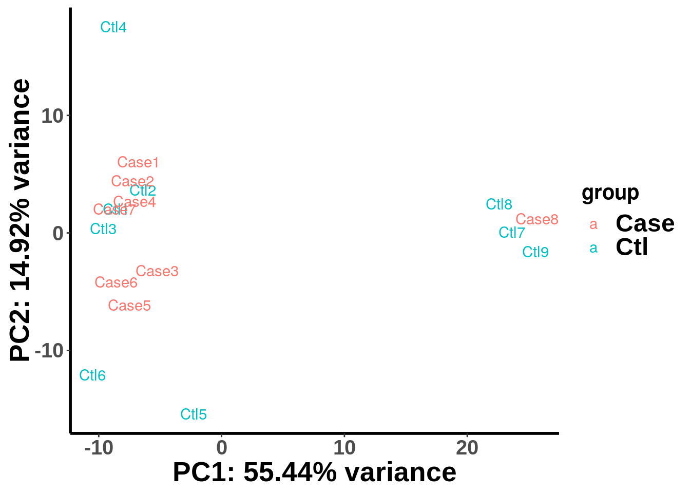
We can see that our Case and Control are not separated by the first two PCs. To check if the samples are separated by batches, we can label the samples by batch instead of by experimental group X.
batch <- c("A","A","A","A","B","B","C","C","C","A","A","B","A","B","B","A","C")
plotPCAfromMatrix(top_bins,group = batch)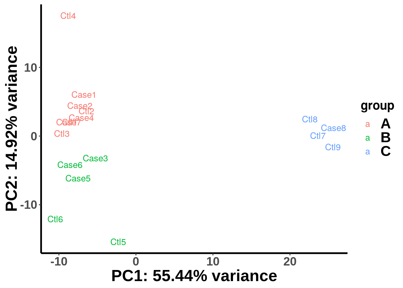
We can see that the samples are clearly separated by batches and we need to account for batch effect in the test. To incorporate covariates in study design, we need first define a covariate matrix table where categorical variable should be converted to (0,1) binary variable.
library(rafalib)
X2 <- as.fumeric(c("A","A","A","A","B","B","A","A","A","A","A","B","A","B","B","A","A"))-1 # batch as covariates
X3 <- as.fumeric(c("A","A","A","A","A","A","C","C","C","A","A","A","A","A","A","A","C"))-1 # batch as covariates
X4 <- as.fumeric(c("M","M","F","M","M","M","F","M","M","M","M","F","M","M","M","M","F"))-1 # sex as covariates
cov <- cbind(X2,X3,X4)

cov
## X2 X3 X4
## [1,] 0 0 0
## [2,] 0 0 0
## [3,] 0 0 1
## [4,] 0 0 0
## [5,] 1 0 0
## [6,] 1 0 0
## [7,] 0 1 1
## [8,] 0 1 0
## [9,] 0 1 0
## [10,] 0 0 0
## [11,] 0 0 0
## [12,] 1 0 1
## [13,] 0 0 0
## [14,] 1 0 0
## [15,] 1 0 0
## [16,] 0 0 0
## [17,] 0 1 1Run the Poisson Gamma test with covariates to account for know source of variation.
radar <- diffIP_parallel(radar,Covariates = cov)or multithread mode
## [1] "The categorical variable has been converted:"
##  Ctl  Ctl  Ctl  Ctl  Ctl  Ctl  Ctl  Ctl  Ctl Case Case Case Case Case Case
##    0    0    0    0    0    0    0    0    0    1    1    1    1    1    1
## Case Case
##    1    1
## running PoissonGamma test at multi-beta mode...
## Hyper-thread registered: TRUE
## Using 10 thread(s) to run multi-beta PoissonGamma test...
## Time used to run multi-beta PoissonGamma test: 0.0140750249226888 mins...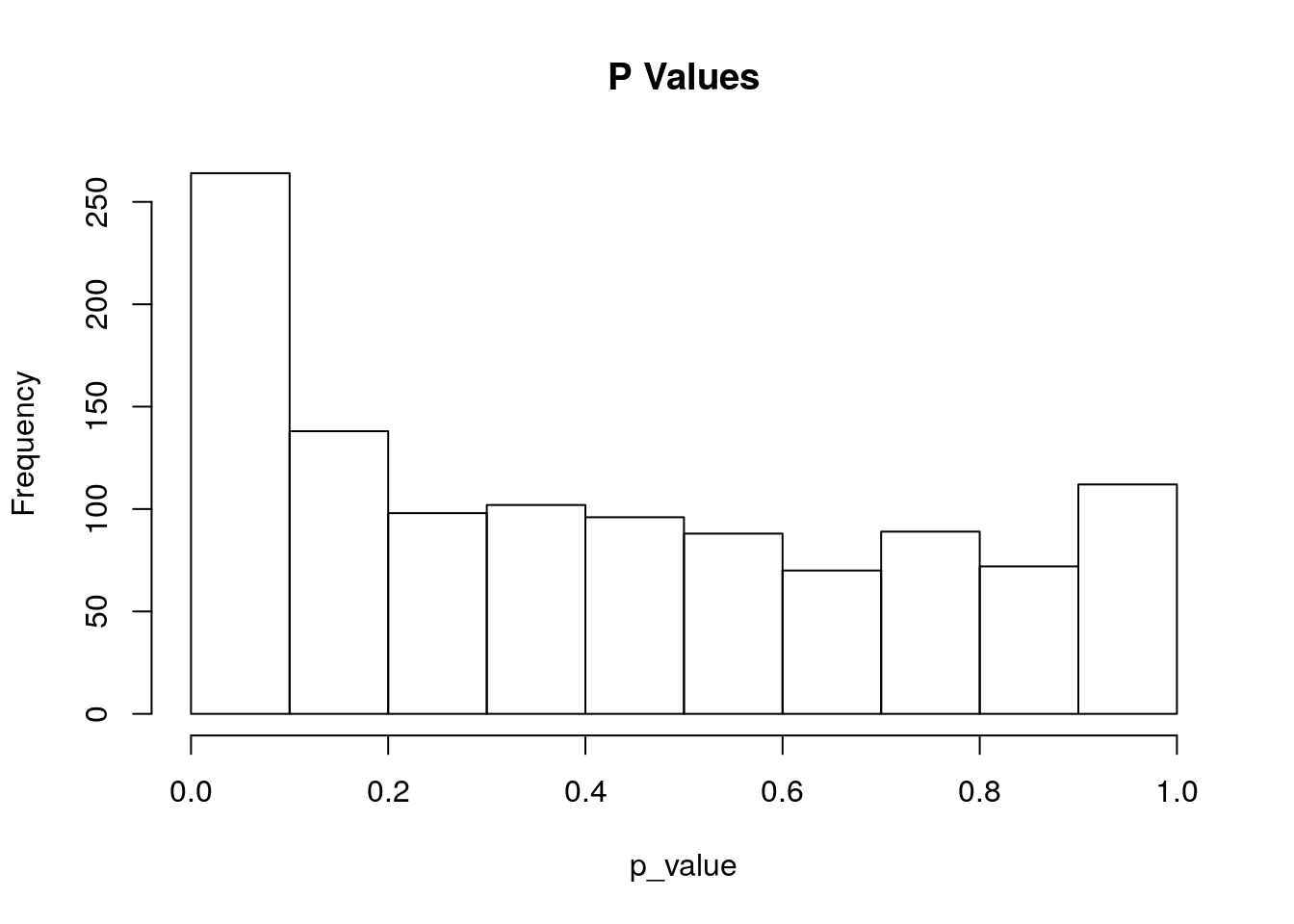
At the end of test, a histgram of p-value distribution will be plotted. The plot can be turned off by diffIP(radar,Covariates = cov,plotPvalue = FALSE).
If for some reasons you want to remove a few samples from the test, you can set index number of the samples you want to skip to exclude them in the Poisson Gamma test.
diffIP_parallel(radar,Covariates = cov,exclude = c() )In the radar object returned by the diffIP(), a mtrix of test estimators has been stored at radar$all.est.
User can check the overall distribution of beta by
hist(radar$all.est[,"beta1"],breaks = 50,main = "Distribution of effect size",xlab = "beta")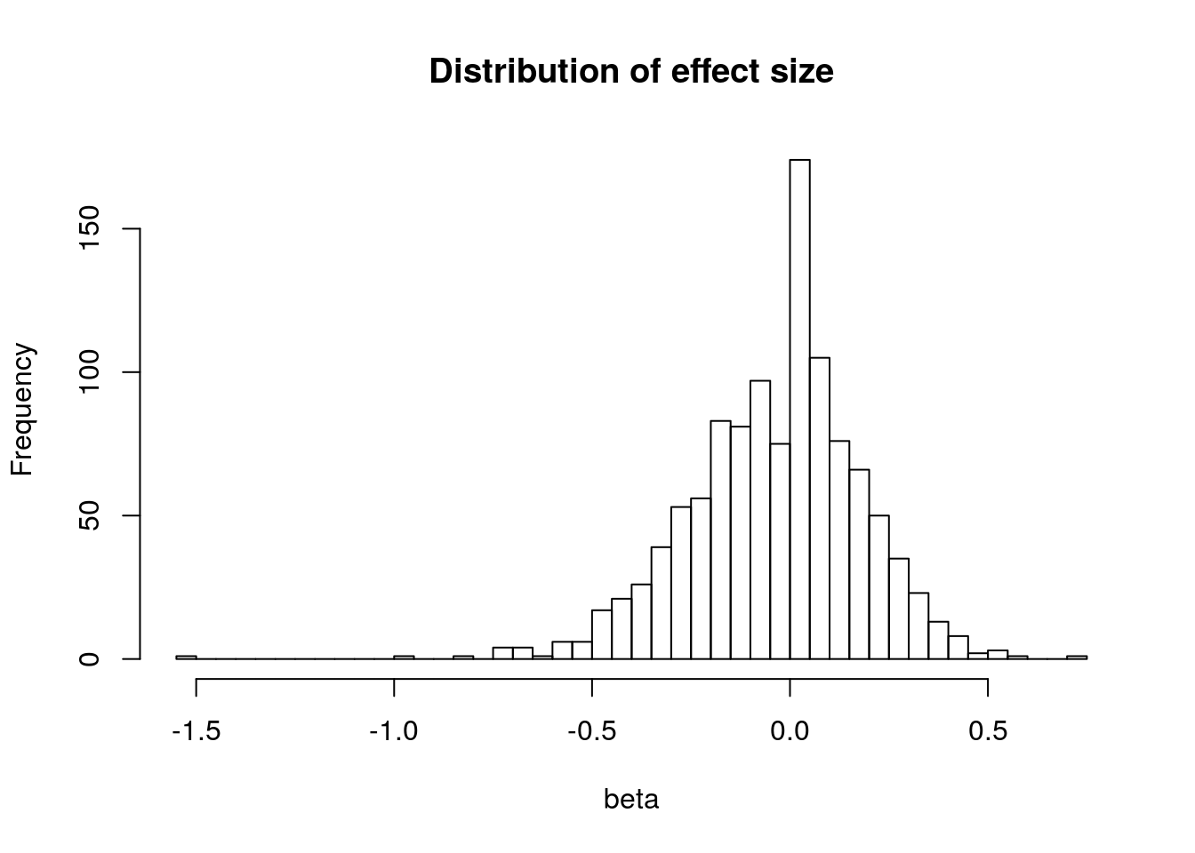
## In case of test without covariates, substitute "beta1" by "beta".g). Visualize the result by heatmap
To assess the pattern of variation of the MeRIP-seq data, we can plot the heatmap of normalized IP read counts adjusted for expression level.
The belowing code shows how to plot heatmap on the radar object.
plotHeatMap(radar)## Plot heat map for top 55 bins ranked by differential test p value...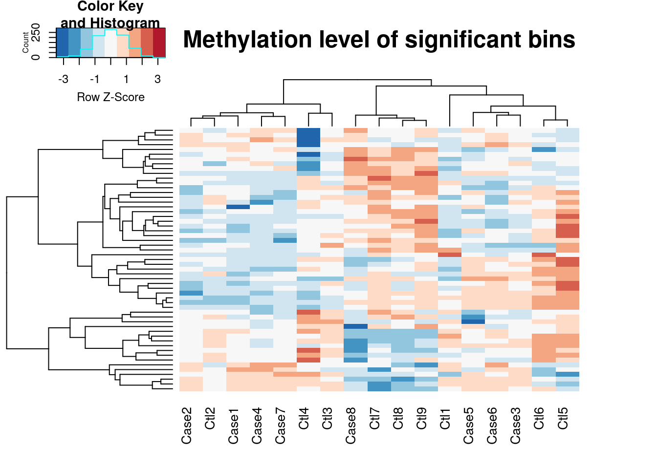
In our example, as we determined earlier by PCA plot that batch effect is contibuting substantially to the variation of our data set. we need to plot heatmap on data regressing out covariates as determined earlier in the analysis. To do so, add covariates matrix to the plotHeatMap() function.
plotHeatMap(radar,covariates = cov)## Plot heat map for top 55 bins ranked by differential test p value...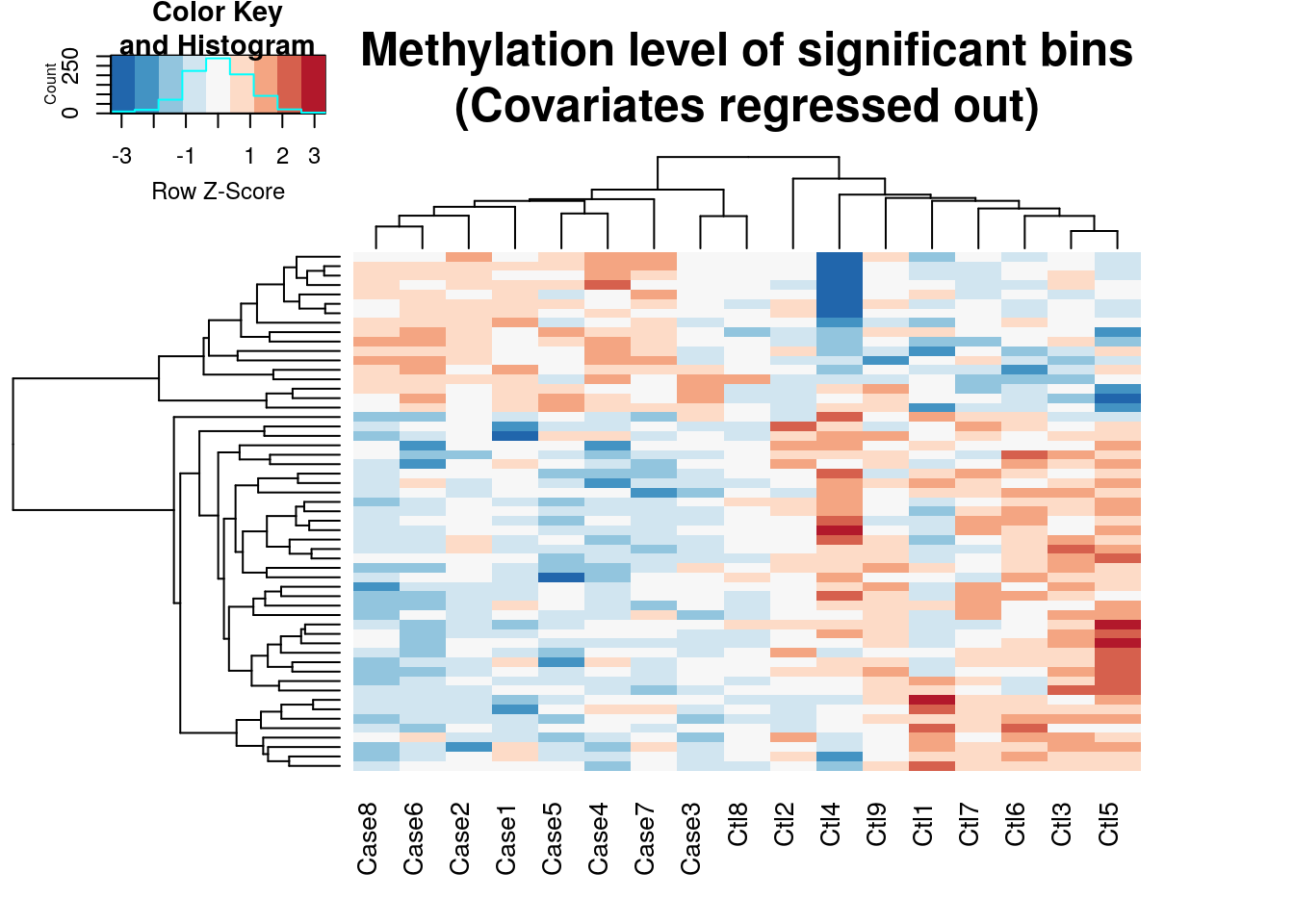
Since plotting too many bins willl look very messy, the function takes the top 5000 bins ranked by test p value. In another words, the heatmap generated here is a visualization the top differential methylated loci. From the heatmap we can see the methylation profile of Ctl8 looks much closer to Cases than to Controls, which suggest this sample is an outlier.
At this point, one can proceed to the next step to report the significantly differentially methylated bins to genomic location or repeat the analysis excluding the outlier sample.
h). Report the result
The count matrix we worked on above are on continuous bins on the transcript and the test was performed on each bin. To report the final result, we want to merge neighbouring bins that pass a significance cutoff because signals for neighbouring bins are assumed to come from the same locus. We merge the p-value of connecting bins by fisher’s method and report the max beta from neighbouring bins. Besides, We also need to report the genomic location instead of on mRNA location of the bin that passed the cutoff. To do so, call the function:
Diff_peak <- reportPoissonGammaMerge(radar,cutoff = 0.05)## Getting significant bins....
## Reporting 11 bins in 10 genes...
## Reporting 11 peaks...
## Hyper-thread registered: TRUE
## Using 6 thread(s) to report merged report...
## Time used to report peaks: 0.00903158585230509 mins...The peak is reported at bed12 format with addition column for beta and p value.
head(Diff_peak)## chr start end name score strand thickStart thickEnd
## 8 chr1 108200159 108200208 SLC25A24 0 - 108200159 108200208
## 10 chr1 110201953 110202002 SLC6A17 0 + 110201953 110202002
## 11 chr1 119623212 119623261 ZNF697 0 - 119623212 119623261
## 5 chr1 120069405 120069454 NOTCH2 0 - 120069405 120069454
## 2 chr1 110212010 110212059 KCNC4 0 + 110212010 110212059
## 9 chr1 110150758 110150807 SLC6A17 0 + 110150758 110150807
## itemRgb blockCount blockSizes blockStarts logFC p_value
## 8 0 1 50 0 -1.5289288 5.824017e-07
## 10 0 1 50 0 -0.9616715 4.658990e-05
## 11 0 1 50 0 -0.7264338 5.017911e-06
## 5 0 1 50 0 -0.7074509 3.333980e-04
## 2 0 1 50 0 -0.7020186 3.099021e-05
## 9 0 1 50 0 -0.6962341 1.055937e-06i). Visualize MeRIP-seq data by sequencing coverage plot.
One of the most straight forward visualization of MeRIP-seq data is the coverage plot. We implemented function to take a radar object and plot the mean/median coverage of IP and INPUT for two inferential groups. Here we demonstrate the function using a differential methylated gene reported in above sections.
To use the plot function, we need to prepare an GTF annotation in GRanges format. This can be done by GTF <- rtracklayer::import("path/to/gtf"). This step only need to be done once in each R session.
GTF <- rtracklayer::import("~/Database/genome/hg38/hg38_UCSC.gtf")
plotGeneCov(radar,geneName = "SLC25A24", center = median, libraryType = "opposite",GTF = GTF)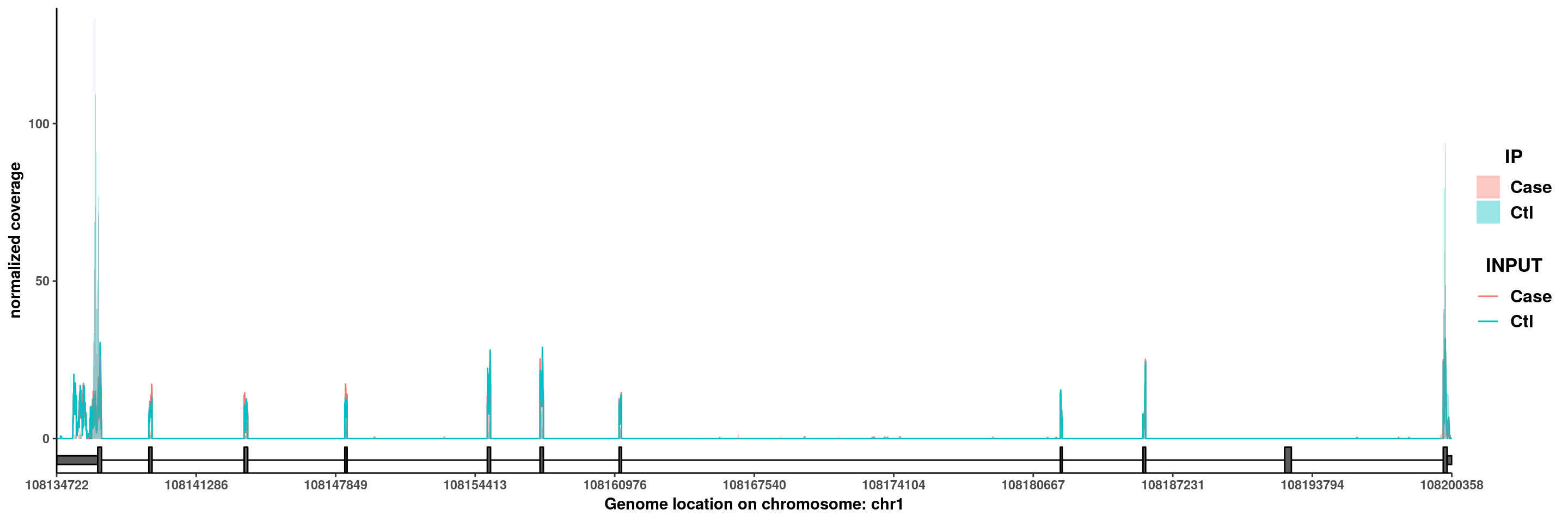
Note The parameter center = median define the coverage to be median of replicates. You can also set it to be center = mean so that the coverage of each group is calculated by taking the mean of replicates.
In some cases, the gene has very long introns that the exon regions becomes too narrow to see in the whole gene plot. We can call the same function with additional parameter ZoomIn to define a range in the gene to plot (Note ZoomIn range need to be within the gene).
plotGeneCov(radar,geneName = "SLC25A24", center = median, libraryType = "opposite",GTF = GTF,ZoomIn = c(108200059,108200308 ) )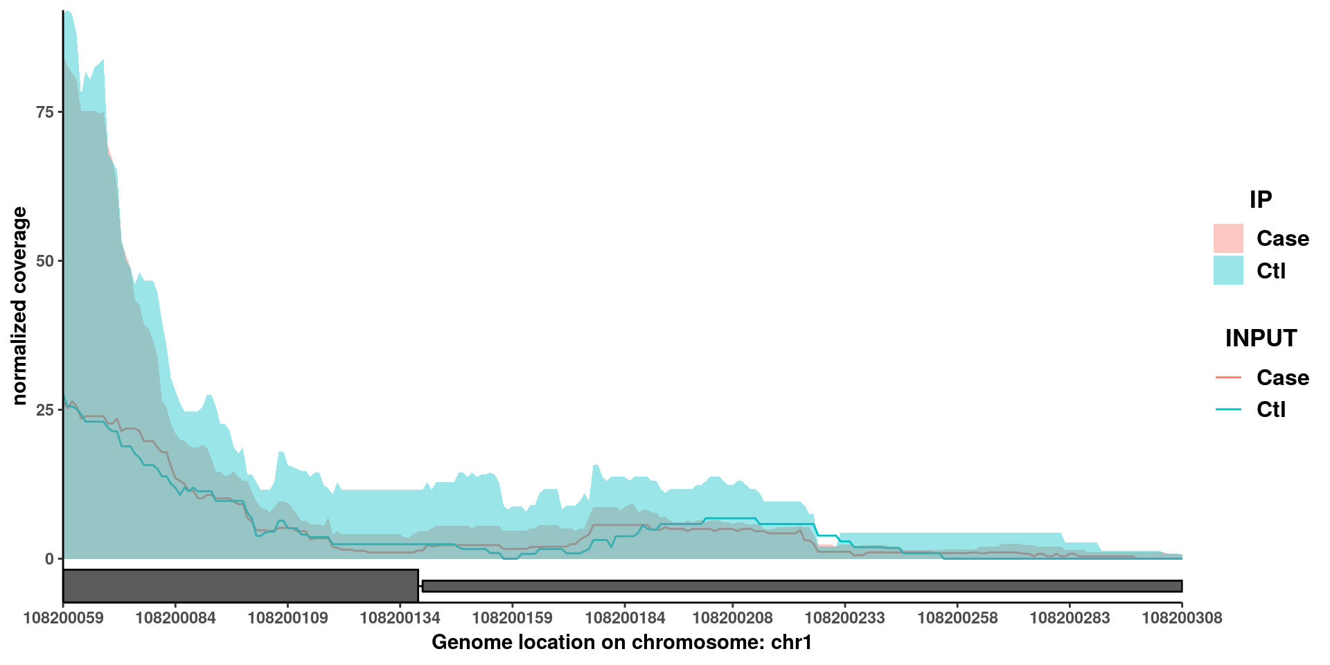
From the coverage plot we can see the in the “Case” group, the m6A peak is significantly decreased.
Another option of plotGeneCov is adjustExprLevel. To facilitate direct comparison of methylation level, by default the plotGeneCov function will adjust/normalize the coverage so that total coverage of this gene is the same for each sample. If you also want to check the expression level difference of the samples by comparing INPUT coverage, this function can be turned off by setting adjustExprLevel = F.
plotGeneCov(radar,geneName = "SLC25A24", center = median, libraryType = "opposite",GTF = GTF,ZoomIn = c(108200059,108200308 ), adjustExprLevel = F )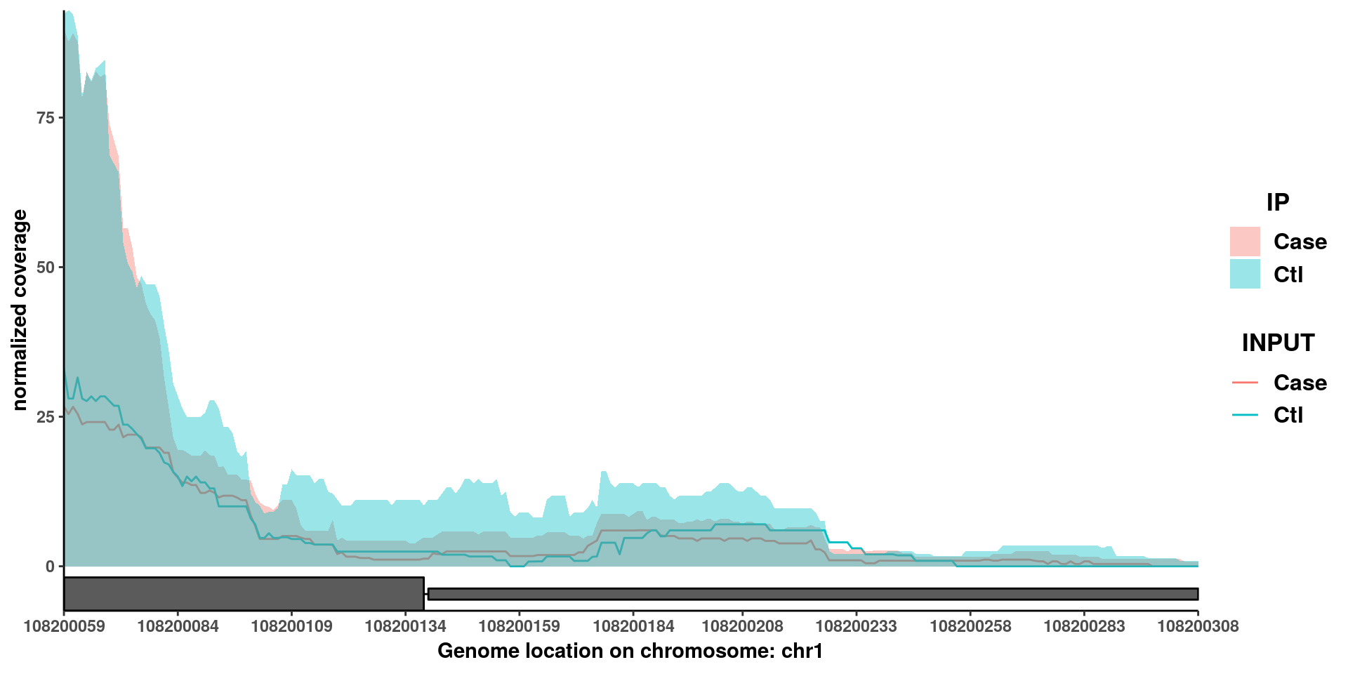
4. Model
a). Poisson model
\[\begin{eqnarray*} Y_{i} &\sim& Poi(\lambda_{i}) \\ \log(\lambda_{i} ) & = & \mu_1 + X_i \beta +e_{i} \end{eqnarray*}\] We assume random effect \(e_{i} \in \log\text{Gamma}(\psi, \psi)\), with scale parameter \(\psi\) and mean equal to \(1\). This is equivalent to \(\lambda_{i} = e^{ \mu_1 + X_i \beta} w_i\) where \(w_i \in \text{Gamma}(\psi, \psi)\) .\[\begin{eqnarray*} P( Y_i | \Theta, - w_i) &=& \int e^{-w_i e^{ \mu_1 + X_i \beta}} \frac{(w_i e^{ \mu_1 + X_i \beta} )^{Y_i}}{Y_i!} \frac{\psi^\psi w_i^{\psi-1}e^{-\psi w_i}}{\Gamma(\psi)} d w_i\\ &=& \frac{ \psi^\psi }{Y_i! } \frac{ \Gamma(Y_i+\psi) } {\Gamma(\psi) } \frac{ (e^{ \mu_1 + X_i \beta})^{Y_i}}{ (e^{ \mu_1 + X_i \beta} + \psi)^{Y_i + \psi}} \end{eqnarray*}\] The marginal log likelihood of observing \(\mathbf{Y}\) can be written as: \[\begin{eqnarray*} \log L( \mathbf{Y} ) &=& \sum_{i}^n [ Y_i( \mu_1 + X_i \beta) + \psi \log \psi + \log \Gamma(Y_i + \psi) - \log Y_i! - \log \Gamma( \psi) - (Y_i + \psi) \log( e^{ \mu_1 + X_i \beta} + \psi)] \\ \end{eqnarray*}\]
b). Estimation
We use gradient ascent algorithm to estimate the parameters, which involves the calculation of first derivatives.\[\begin{eqnarray*} \frac{ \partial \log L( \mathbf{Y} ) }{ \partial \beta } &=& \sum_{i}^n \ \Big[ Y_i - \big (Y_i + \psi \big )\frac{e^{ \mu_1+ X_i \beta}}{ e^{ \mu_1 + X_i \beta} +\psi} \Big] X_i \\ \frac{ \partial \log L( \mathbf{Y} ) }{ \partial \psi} &=& \sum_{i}^n \Big [ \log \psi + 1 - \frac{Y_i + \psi }{ e^{ \mu_1 + X_i \beta} +\psi} - \log ( e^{ \mu_1 + X_i \beta} +\psi ) \\ &&+ \text{digamma} ( Y_i + \psi) - \text{digamma} ( \psi) \Big ] \\ \frac{ \partial \log L( \mathbf{Y} ) }{ \partial \mu _1} &=& \sum_{i}^n \Big[ Y_i - \big (Y_i + \psi \big ) \frac{e^{ \mu_1 + X_i \beta} }{e^{ \mu_1 + X_i \beta} + \psi} \Big] \end{eqnarray*}\]
In each iteration, the parameters are updated through $ {(t+1)} = {(t)} + s_{(t+1)} _ {|= _{(t)}}$. The step size \(s_{(t+1)}\) is determined by a line search algorithm.
c). Inference
We use log-likelihood ratio test to make the inference, where the null model is \[\begin{eqnarray*} Y_{i} &\sim& Poi(\lambda_{i}) \\ \log(\lambda_{i} ) & = & \mu_1 + e_{i}. \end{eqnarray*}\]d). Poisson model + covariates
\[\begin{eqnarray*} Y_{i} &\sim& Poi(\lambda_{i}) \\ \log(\lambda_{i} ) & = & \mu_1 + \mathbf{X_i} \mathbf{\beta} +e_{i} \end{eqnarray*}\]We assume random effect \(e_{i} \in \log\text{Gamma}(\psi, \psi)\), with scale parameter \(\psi\) and mean equal to \(1\). This is equivalent to \(\lambda_{i} = e^{ \mu_1 + \mathbf{X_i} \mathbf{\beta}} w_i\) where \(w_i \in \text{Gamma}(\psi, \psi)\) .
\[\begin{eqnarray*} P( Y_i | \Theta, - w_i) &=& \int e^{-w_i e^{ \mu_1 + \mathbf{X_i} \mathbf{\beta}}} \frac{(w_i e^{ \mu_1 + \mathbf{X_i} \mathbf{\beta}} )^{Y_i}}{Y_i!} \frac{\psi^\psi w_i^{\psi-1}e^{-\psi w_i}}{\Gamma(\psi)} d w_i\\ &=& \frac{ \psi^\psi }{Y_i! } \frac{ \Gamma(Y_i+\psi) } {\Gamma(\psi) } \frac{ (e^{ \mu_1 + \mathbf{X_i} \mathbf{\beta}})^{Y_i}}{ (e^{ \mu_1 + \mathbf{X_i} \mathbf{\beta}} + \psi)^{Y_i + \psi}} \end{eqnarray*}\] The marginal log likelihood of observing \(\mathbf{Y}\) can be written as: \[\begin{eqnarray*} \log L( \mathbf{Y} ) &=& \sum_{i}^n [ Y_i( \mu_1 + \mathbf{X_i} \mathbf{\beta} ) + \psi \log \psi + \log \Gamma(Y_i + \psi) - \log Y_i! - \log \Gamma( \psi) - (Y_i + \psi) \log( e^{ \mu_1 + \mathbf{X_i} \mathbf{\beta}} + \psi)] \\ \end{eqnarray*}\]Estimation
We use gradient ascent algorithm to estimate the parameters, which involves the calculation of first derivatives.\[\begin{eqnarray*} \frac{ \partial \log L( \mathbf{Y} ) }{ \partial \beta_k } &=& \sum_{i}^n \ \Big[ Y_i - \big (Y_i + \psi \big )\frac{e^{ \mu_1+ \mathbf{X_i} \mathbf{\beta}}}{ e^{ \mu_1 + \mathbf{X_i} \mathbf{\beta}} +\psi} \Big] X_{ik} \\ \frac{ \partial \log L( \mathbf{Y} ) }{ \partial \psi} &=& \sum_{i}^n \Big [ \log \psi + 1 - \frac{Y_i + \psi }{ e^{ \mu_1 + \mathbf{X_i} \mathbf{\beta} } +\psi} - \log ( e^{ \mu_1 + \mathbf{X_i} \mathbf{\beta}} +\psi ) \\ &&+ \text{digamma} ( Y_i + \psi) - \text{digamma} ( \psi) \Big ] \\ \frac{ \partial \log L( \mathbf{Y} ) }{ \partial \mu _1} &=& \sum_{i}^n \Big[ Y_i - \big (Y_i + \psi \big ) \frac{e^{ \mu_1 + \mathbf{X_i} \mathbf{\beta}} }{e^{ \mu_1 + \mathbf{X_i} \mathbf{\beta}} + \psi} \Big] \end{eqnarray*}\]
In each iteration, the parameters are updated through $ {(t+1)} = {(t)} + s_{(t+1)} _ {|= _{(t)}}$. The step size \(s_{(t+1)}\) is determined by a line search algorithm.
Inference
We use log-likelihood ratio test to make the inference for each \(\beta_k\), where the null model is \[\begin{eqnarray*} Y_{i} &\sim& Poi(\lambda_{i}) \\ \log(\lambda_{i} ) & = & \mu_1 + \sum_{j \neq k}^{K} X_{ij} \beta_j + e_{i}. \end{eqnarray*}\] We use observed fisher information to make the inference for all parameters. The calculation involves all second derivatives and partial derivatives.\[\begin{eqnarray*} \frac{ \partial^2\log L( \mathbf{Y} )}{\partial \beta_k^2} &=& - \sum_{i}^n \frac{e^{ \mu_1 + \mathbf{X_i} \mathbf{\beta} }}{ \big ( e^{ \mu_1 + \mathbf{X_i} \mathbf{\beta} } + \psi \big ) ^2} \psi \big (Y_i + \psi \big ) X_{ik}^2 \\ \frac{ \partial^2\log L( \mathbf{Y} )}{\partial \beta_k \beta_k'} &=& - \sum_{i}^n \frac{e^{ \mu_1 + \mathbf{X_i} \mathbf{\beta} }}{ \big ( e^{ \mu_1 + \mathbf{X_i} \mathbf{\beta} } + \psi \big ) ^2} \psi \big (Y_i + \psi \big ) X_{ik} X_{ik'} \\ \frac{ \partial^2 \log L( \mathbf{Y} ) }{\partial \beta_k \partial \mu_1} &=& - \sum_{i}^n \frac{e^{ \mu_1 + \mathbf{X_i} \mathbf{\beta} }}{ \big ( e^{ \mu_1 + \mathbf{X_i} \mathbf{\beta} } + \psi \big ) ^2} \psi \big (Y_i + \psi \big ) X_{ik} \\ \frac{ \partial^2 \log L( \mathbf{Y} ) }{\partial \beta_k \partial \psi} &=& \sum_{i}^n \Big[ \frac{e^{ \mu_1 + \mathbf{X_i} \mathbf{\beta} } }{ \big ( e^{ \mu_1 + \mathbf{X_i} \mathbf{\beta} } + \psi \big ) ^2} \big (Y_i + \psi \big ) X_{ik} - \frac{e^{ \mu_1 + \mathbf{X_i} \mathbf{\beta} } }{ e^{ \mu_1 + \mathbf{X_i} \mathbf{\beta} } + \psi } X_{ik} \Big]\\ \frac{ \partial^2 \log L( \mathbf{Y} ) }{\partial \mu_1^2} &=& - \sum_{i}^n \frac{e^{ \mu_1 + \mathbf{X_i} \mathbf{\beta}} }{ \big ( e^{ \mu_1 + \mathbf{X_i} \mathbf{\beta} } + \psi \big ) ^2} \psi \big (Y_i + \psi \big ) \\ \frac{ \partial^2 \log L( \mathbf{Y} ) }{\partial \mu_1 \partial \psi} &=& \sum_{i}^n \Big[ \frac{e^{ \mu_1 + \mathbf{X_i} \mathbf{\beta} } }{ \big ( e^{ \mu_1 + \mathbf{X_i} \mathbf{\beta} } + \psi \big ) ^2} \big (Y_i + \psi \big ) -\frac{e^{ \mu_1 + \mathbf{X_i} \mathbf{\beta} } }{ e^{ \mu_1 + \mathbf{X_i} \mathbf{\beta} } + \psi } \Big] \\ \frac{ \partial^2 \log L( \mathbf{Y} ) }{\partial \psi^2} &=& \sum_{i}^n \Big[ \frac{1}{\psi} - \frac{2}{e^{ \mu_1 + \mathbf{X_i} \mathbf{\beta} } + \psi} + \frac{Y_i + \psi }{ \big ( e^{ \mu_1 + \mathbf{X_i} \mathbf{\beta}} + \psi \big ) ^2} + \text{trigamma}(Y_i + \psi) - \text{trigamma}(\psi) \Big] \\ \end{eqnarray*}\]
Session info
sessionInfo()## R version 3.5.0 (2018-04-23)
## Platform: x86_64-pc-linux-gnu (64-bit)
## Running under: Ubuntu 17.10
##
## Matrix products: default
## BLAS: /usr/lib/x86_64-linux-gnu/openblas/libblas.so.3
## LAPACK: /usr/lib/x86_64-linux-gnu/libopenblasp-r0.2.20.so
##
## locale:
## [1] LC_CTYPE=en_US.UTF-8 LC_NUMERIC=C
## [3] LC_TIME=en_US.UTF-8 LC_COLLATE=en_US.UTF-8
## [5] LC_MONETARY=en_US.UTF-8 LC_MESSAGES=en_US.UTF-8
## [7] LC_PAPER=en_US.UTF-8 LC_NAME=C
## [9] LC_ADDRESS=C LC_TELEPHONE=C
## [11] LC_MEASUREMENT=en_US.UTF-8 LC_IDENTIFICATION=C
##
## attached base packages:
## [1] stats4 parallel stats graphics grDevices utils datasets
## [8] methods base
##
## other attached packages:
## [1] rafalib_1.0.0 RADAR_0.1.5
## [3] RcppArmadillo_0.9.200.4.0 Rcpp_1.0.0
## [5] RColorBrewer_1.1-2 gplots_3.0.1
## [7] doParallel_1.0.14 iterators_1.0.10
## [9] foreach_1.4.4 ggplot2_3.1.0
## [11] Rsamtools_1.34.0 Biostrings_2.50.1
## [13] XVector_0.22.0 GenomicFeatures_1.34.1
## [15] AnnotationDbi_1.44.0 Biobase_2.42.0
## [17] GenomicRanges_1.34.0 GenomeInfoDb_1.18.1
## [19] IRanges_2.16.0 S4Vectors_0.20.1
## [21] BiocGenerics_0.28.0
##
## loaded via a namespace (and not attached):
## [1] bitops_1.0-6 matrixStats_0.54.0
## [3] bit64_0.9-7 progress_1.2.0
## [5] httr_1.3.1 rprojroot_1.3-2
## [7] tools_3.5.0 backports_1.1.2
## [9] R6_2.3.0 rpart_4.1-13
## [11] KernSmooth_2.23-15 Hmisc_4.1-1
## [13] DBI_1.0.0 lazyeval_0.2.1
## [15] colorspace_1.3-2 nnet_7.3-12
## [17] withr_2.1.2 gridExtra_2.3
## [19] tidyselect_0.2.5 prettyunits_1.0.2
## [21] DESeq2_1.22.1 bit_1.1-14
## [23] compiler_3.5.0 htmlTable_1.12
## [25] DelayedArray_0.8.0 labeling_0.3
## [27] rtracklayer_1.42.1 checkmate_1.8.5
## [29] caTools_1.17.1.1 scales_1.0.0
## [31] genefilter_1.64.0 stringr_1.3.1
## [33] digest_0.6.18 foreign_0.8-71
## [35] rmarkdown_1.10 base64enc_0.1-3
## [37] pkgconfig_2.0.2 htmltools_0.3.6
## [39] htmlwidgets_1.3 rlang_0.3.0.1
## [41] rstudioapi_0.8 RSQLite_2.1.1
## [43] bindr_0.1.1 BiocParallel_1.16.1
## [45] gtools_3.8.1 acepack_1.4.1
## [47] dplyr_0.7.8 RCurl_1.95-4.11
## [49] magrittr_1.5 GenomeInfoDbData_1.2.0
## [51] Formula_1.2-3 Matrix_1.2-15
## [53] munsell_0.5.0 stringi_1.2.4
## [55] yaml_2.2.0 SummarizedExperiment_1.12.0
## [57] zlibbioc_1.28.0 qvalue_2.14.0
## [59] plyr_1.8.4 grid_3.5.0
## [61] blob_1.1.1 gdata_2.18.0
## [63] crayon_1.3.4 lattice_0.20-38
## [65] splines_3.5.0 annotate_1.60.0
## [67] hms_0.4.2 locfit_1.5-9.1
## [69] knitr_1.20 pillar_1.3.0
## [71] reshape2_1.4.3 geneplotter_1.60.0
## [73] codetools_0.2-15 biomaRt_2.38.0
## [75] XML_3.98-1.16 glue_1.3.0
## [77] evaluate_0.12 latticeExtra_0.6-28
## [79] data.table_1.11.8 BiocManager_1.30.4
## [81] gtable_0.2.0 purrr_0.2.5
## [83] assertthat_0.2.0 xtable_1.8-3
## [85] survival_2.43-1 tibble_1.4.2
## [87] GenomicAlignments_1.18.0 memoise_1.1.0
## [89] bindrcpp_0.2.2 cluster_2.0.7-1
## [91] BiocStyle_2.10.0References
[1] Love, M. I.; Huber, W.; & Anders, S. Moderated estimation of fold change and dispersion for RNA-seq data with DESeq2. Genome Biology. 2014 15(12), 550.
This R Markdown site was created with workflowr