T2D

Count reads

library(RADAR)

samplenames = c("Ctl1","Ctl4","Ctl8","Ctl16","Ctl17","Ctl18","Ctl20","T2D1","T2D4","T2D5","T2D6","T2D7","T2D9","T2D11","T2D12")

RADAR <- countReads(samplenames = samplenames,
                    gtf = "~/Database/genome/hg38/hg38_UCSC.gtf",
                    bamFolder = "~/Rohit_T2D/bam_files",
                    outputDir =  "~/Rohit_T2D",
                    modification = "IP",
                    threads = 25
)

monster <- RADAR

Summary of read count

library(RADAR)
library(qvalue)
#load("~/Rohit_T2D/RADAR.RData")
load("~/Rohit_T2D/RADAR_analysis.RData")
countSummary <- rbind("Input"= colSums(RADAR$reads)[1:length(RADAR$samplenames)], "IP" =colSums(RADAR$reads)[(1:length(RADAR$samplenames))+length(RADAR$samplenames)] )
colnames(countSummary) <- RADAR$samplenames
knitr::kable(countSummary,format = "pandoc" )

	Ctl1	Ctl4	Ctl8	Ctl16	Ctl17	Ctl18	Ctl20	T2D1	T2D4	T2D5	T2D6	T2D7	T2D9	T2D11	T2D12
Input	18320414	17749453	17923796	11508719	15118237	25923296	20302596	16803517	16105448	14146820	17202593	14336611	17758817	19782144	18779123
IP	30287782	25105375	21908869	23197918	21409901	31653712	24753657	27733641	26634012	28457739	22539106	36100747	27434039	22053013	19402847

X <- c(rep("Ctl",7),rep("T2D",8))
RADAR <- normalizeLibrary(RADAR,X)
RADAR <- RADAR::adjustExprLevel(RADAR)
RADAR <- filterBins(RADAR,minCountsCutOff = 15)

RADAR_pos <- RADAR::adjustExprLevel(RADAR[1:12], adjustBy = "pos")
RADAR_pos <- filterBins(RADAR_pos,minCountsCutOff = 15)

INPUT read count

Local INPUT read count

Plot distribution of number of reads in each 50 bp bins

hist(log10(rowMeans(RADAR$reads[rowMeans(RADAR$reads[,grep("input",colnames(RADAR$reads))])>1,grep("input",colnames(RADAR$reads))])  ),xlab = "log10 read count",main = "Distribution of INPUT read count in bins",xlim = c(0,3), col =rgb(0.2,0.2,0.2,0.5),cex.main = 2,cex.axis =2,cex.lab=2)
axis(side = 1, lwd = 2,cex.axis =2)
axis(side = 2, lwd = 2,cex.axis =2)

local read count V.S. geneSum

Compute the within group variability of INPUT geneSum VS INPUT local read count.

var.coef <- function(x){sd(as.numeric(x))/mean(as.numeric(x))}
## filter expressed genes
geneSum <- RADAR$geneSum[rowSums(RADAR$geneSum)>16,]
## within group variability
relative.var <- t( apply(geneSum,1,tapply,RADAR$X,var.coef) )
geneSum.var <- c(relative.var)

## For each gene used above, random sample a 50bp bin within this gene
set.seed(1)
r.bin50 <- tapply(rownames(RADAR$norm.input)[which(RADAR$geneBins$gene %in% rownames(geneSum))],as.character( RADAR$geneBins$gene[which(RADAR$geneBins$gene %in% rownames(geneSum))]) ,function(x){
  n <- sample(1:length(x),1)
  return(x[n])
})

relative.var <- apply(RADAR$norm.input[r.bin50,],1,tapply,RADAR$X,var.coef)
bin50.var <- c(relative.var)
bin50.var <- bin50.var[!is.na(bin50.var)]

## 100bp bins
r.bin100 <- tapply(rownames(RADAR$norm.input)[which(RADAR$geneBins$gene %in% rownames(geneSum))],as.character( RADAR$geneBins$gene[which(RADAR$geneBins$gene %in% rownames(geneSum))]) ,function(x){
  n <- sample(1:(length(x)-2),1)
  return(x[n:(n+1)])
})
relative.var <- lapply(r.bin100, function(x){ tapply( colSums(RADAR$norm.input[x,]),RADAR$X,var.coef ) })
bin100.var <- unlist(relative.var)
bin100.var <- bin100.var[!is.na(bin100.var)]

## 200bp bins
r.bin200 <- tapply(rownames(RADAR$norm.input)[which(RADAR$geneBins$gene %in% rownames(geneSum))],as.character( RADAR$geneBins$gene[which(RADAR$geneBins$gene %in% rownames(geneSum))]) ,function(x){
  if(length(x)>4){
    n <- sample(1:(length(x)-3),1)
    return(x[n:(n+3)])
  }else{
    return(NULL)
  }
})
r.bin200 <- r.bin200[which(!unlist(lapply(r.bin200,is.null)) ) ]
relative.var <- lapply(r.bin200, function(x){ tapply( colSums(RADAR$norm.input[x,]),RADAR$X,var.coef ) })

bin200.var <- unlist(relative.var)
bin200.var <- bin200.var[!is.na(bin200.var)]

relative.var <- data.frame(group=c(rep("geneSum",length(geneSum.var)),rep("bin-50bp",length(bin50.var)),rep("bin-100bp",length(bin100.var)),rep("bin-200bp",length(bin200.var))), variance=c(geneSum.var,bin50.var,bin100.var,bin200.var))

ggplot(relative.var,aes(variance,colour=group))+geom_density()+xlab("Relative variation")+
  theme_bw() + theme(panel.border = element_blank(), panel.grid.major = element_blank(),
                   panel.grid.minor = element_blank(), axis.line = element_line(colour = "black",size = 1),
                   axis.title.x=element_text(size=20, face="bold", hjust=0.5,family = "arial"),
                   axis.title.y=element_text(size=20, face="bold", vjust=0.4, angle=90,family = "arial"),
                   legend.position = c(0.88,0.88),legend.title=element_blank(),legend.text = element_text(size = 14, face = "bold",family = "arial"),
                   axis.text = element_text(size = 15,face = "bold",family = "arial",colour = "black")  )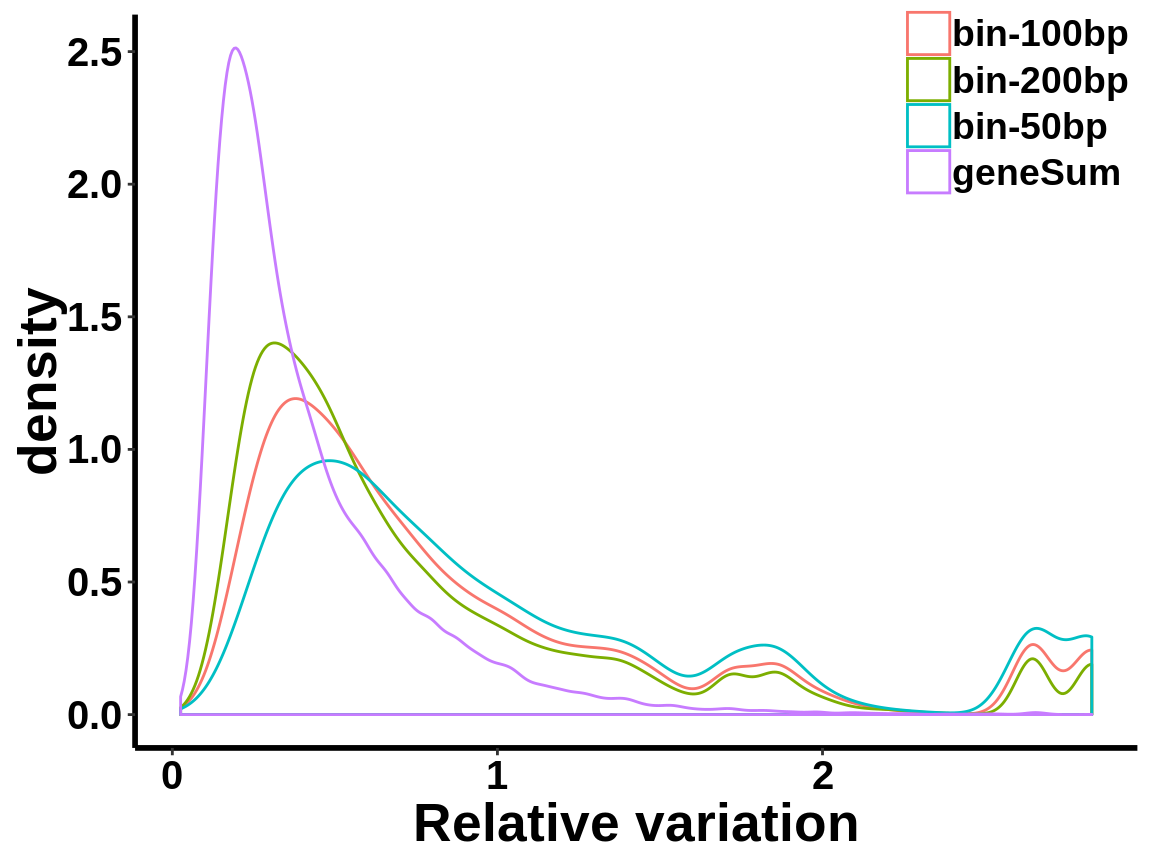

Compare MeRIP-seq IP data with regular RNA-seq data

var.coef <- function(x){sd(as.numeric(x))/mean(as.numeric(x))}

ip_coef_var <- t(apply(RADAR$ip_adjExpr_filtered,1,tapply,X,var.coef))
ip_coef_var <- ip_coef_var[!apply(ip_coef_var,1,function(x){return(any(is.na(x)))}),]
#hist(c(ip_coef_var),main = "M14KO mouse liver\n m6A-IP",xlab = "within group coefficient of variation",breaks = 50)
###
gene_coef_var <-  t(apply(RADAR$geneSum,1,tapply,X,var.coef))
gene_coef_var <- gene_coef_var[!apply(gene_coef_var,1,function(x){return(any(is.na(x)))}),]
#hist(c(gene_coef_var),main = "M14KO mouse liver\n RNA-seq",xlab = "within group coefficient of variation",breaks = 50)

coef_var <- list('RNA-seq'=c(gene_coef_var),'m6A-IP'=c(ip_coef_var))
nn<-sapply(coef_var, length)
rs<-cumsum(nn)
re<-rs-nn+1
grp <- factor(rep(names(coef_var), nn), levels=names(coef_var))
coef_var.df <- data.frame(coefficient_var = c(c(gene_coef_var),c(ip_coef_var)),label = grp)

ggplot(data = coef_var.df,aes(coefficient_var,colour = grp))+geom_density()+  theme_bw() + theme(panel.border = element_blank(), panel.grid.major = element_blank(),
                   panel.grid.minor = element_blank(), axis.line = element_line(colour = "black",size = 1),
                   axis.title.x=element_text(size=20, face="bold", hjust=0.5,family = "arial"),
                   axis.title.y=element_text(size=20, face="bold", vjust=0.4, angle=90,family = "arial"),
                   legend.position = c(0.9,0.9),legend.title=element_blank(),legend.text = element_text(size = 18, face = "bold",family = "arial"),
                   axis.text = element_text(size = 15,face = "bold",family = "arial",colour = "black")   )+
  xlab("Coefficient of variation")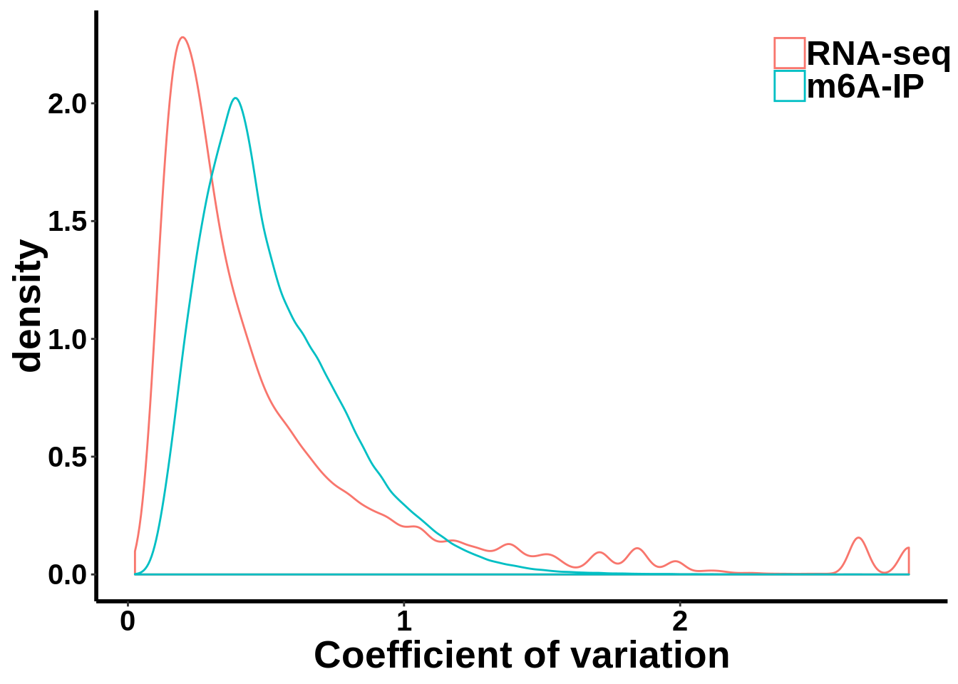

Check mean variance relationship of the data.

ip_var <- t(apply(RADAR$ip_adjExpr_filtered,1,tapply,X,var))
#ip_var <- ip_coef_var[!apply(ip_var,1,function(x){return(any(is.na(x)))}),]
ip_mean <- t(apply(RADAR$ip_adjExpr_filtered,1,tapply,X,mean))

###
gene_var <-  t(apply(RADAR$geneSum,1,tapply,X,var))
#gene_var <- gene_var[!apply(gene_var,1,function(x){return(any(is.na(x)))}),]
gene_mean <- t(apply(RADAR$geneSum,1,tapply,X,mean))

all_var <- list('RNA-seq'=c(gene_var),'m6A-IP'=c(ip_var))
nn<-sapply(all_var, length)
rs<-cumsum(nn)
re<-rs-nn+1
group <- factor(rep(names(all_var), nn), levels=names(all_var))
all_var.df <- data.frame(variance = c(c(gene_var),c(ip_var)),mean= c(c(gene_mean),c(ip_mean)),label = group)

ggplot(data = all_var.df,aes(x=mean,y=variance,colour = group,shape = group))+geom_point(size = I(0.2))+stat_smooth(se = T,show.legend = F)+stat_smooth(se = F)+theme_bw() +xlab("Mean")+ylab("Variance") +theme(panel.border = element_blank(), panel.grid.major = element_blank(),
                   panel.grid.minor = element_blank(), axis.line = element_line(colour = "black",size = 1),
                   axis.title.x=element_text(size=22, face="bold", hjust=0.5,family = "arial"),
                   axis.title.y=element_text(size=22, face="bold", vjust=0.4, angle=90,family = "arial"),
                   legend.position = c(0.85,0.95),legend.title=element_blank(),legend.text = element_text(size = 20, face = "bold",family = "arial"),
                   axis.text = element_text(size = 15,face = "bold",family = "arial",colour = "black") ) +
  scale_x_continuous(limits = c(0,5000))+scale_y_continuous(limits = c(0,4e6))

inputCount <- as.data.frame(RADAR$reads[,1:length(RADAR$samplenames)])
logInputCount <- as.data.frame(log( RADAR$geneSum  )  )

ggplot(logInputCount, aes(x = `Ctl18` , y = `T2D6` ))+geom_point()+geom_abline(intercept = 0,slope = 1, lty = 2, colour = "red")+xlab(paste("Log counts Ctl18") )+ylab(paste("Log counts T2D6") )+theme_classic(base_line_size = 0.8)+theme(axis.title = element_text(size = 12,face = "bold"), axis.text =  element_text(size = 10,face = "bold",colour = "black") )

ggplot(logInputCount, aes(x = `Ctl18` , y = `T2D5` ))+geom_point()+geom_abline(intercept = 0,slope = 1, lty = 2, colour = "red")+xlab(paste("Log counts Ctl18") )+ylab(paste("Log counts T2D5") )+theme_classic(base_line_size = 0.8)+theme(axis.title = element_text(size = 12,face = "bold"), axis.text =  element_text(size = 10,face = "bold",colour = "black") )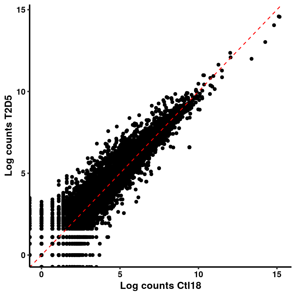

PCA analysis

After geting the filtered and normalized IP read count for testing, we can use PCA analysis to check unkown variation.

top_bins <- RADAR$ip_adjExpr_filtered[order(rowMeans(RADAR$ip_adjExpr_filtered))[1:15000],]

We plot PCA colored by Ctl vs T2D

plotPCAfromMatrix(top_bins,group = X)+scale_color_discrete(name = "Group")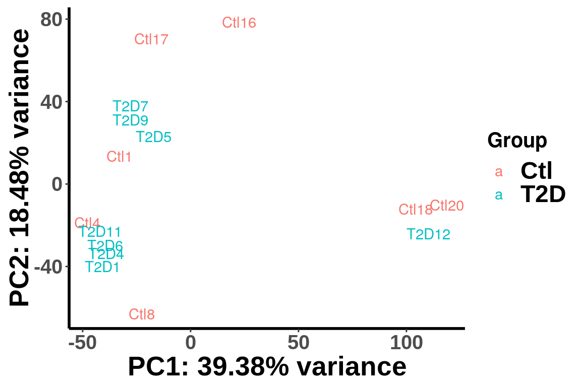

(Norm by position)

plotPCAfromMatrix(RADAR_pos$ip_adjExpr_filtered[order(rowMeans(RADAR_pos$ip_adjExpr_filtered))[1:15000],],group = X )+scale_color_discrete(name = "Group")

To check if samples are separated by different sequencing lanes, label the samples by lane batch.

batch <- c("A","A","A","B","B","C","C","A","A","B","A","B","B","A","C")
plotPCAfromMatrix(top_bins,group = paste0(batch))+scale_color_discrete(name = "Batch")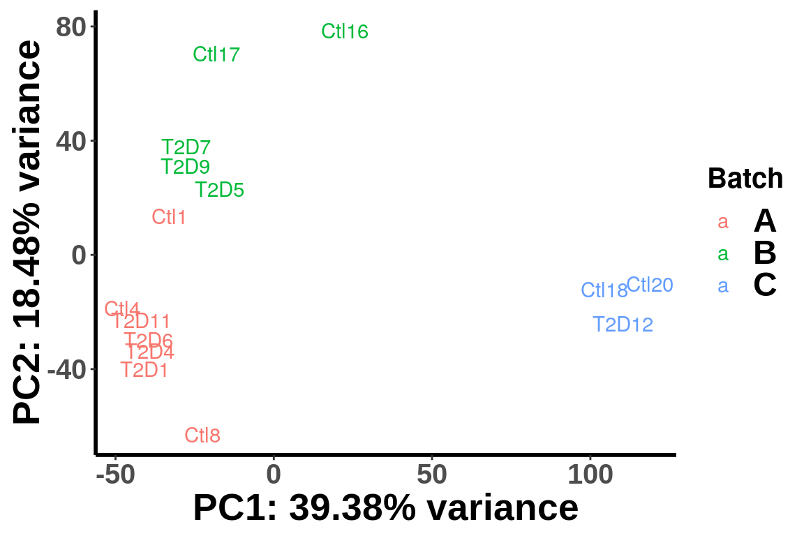

We can see that the samples are clearly separated by batches and we need to account for batch effect in the test. Thus we incorporate batch and gender as known covariates in the test.

Check the PCA after r egressing out the batch and gender.

library(rafalib)
X2 <- as.fumeric(c("A","A","A","B","B","A","A","A","A","B","A","B","B","A","A"))-1 # batch as covariates
X3 <- as.fumeric(c("A","A","A","A","A","C","C","A","A","A","A","A","A","A","C"))-1 # batch as covariates
X4 <- as.fumeric(c("M","F","M","M","M","F","M","M","M","F","M","M","M","M","F"))-1 # sex as covariates
registerDoParallel(cores = 10)
m6A.cov.out <- foreach(i = 1:nrow(top_bins), .combine = rbind) %dopar% {
  Y = top_bins[i,]
  resi <- residuals( lm(log(Y+1) ~ X2 + X3 + X4 ) )
  resi
}
rm(list=ls(name=foreach:::.foreachGlobals), pos=foreach:::.foreachGlobals)
rownames(m6A.cov.out) <- rownames(top_bins)

plotPCAfromMatrix(m6A.cov.out,X,loglink = FALSE)+scale_color_discrete(name = "Group")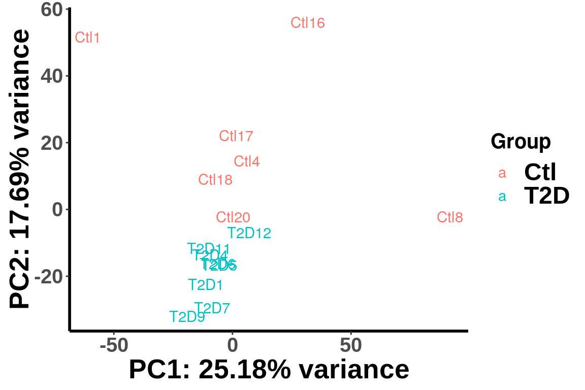

After regressing out the covariates, the samples are separated by diseases status in the PCA plot.

Run PoissonGamma test

cov <- cbind(X2,X3,X4)
RADAR <-  diffIP_parallel(RADAR,Covariates = cov,thread = 20)
RADAR_pos <-  diffIP_parallel(RADAR_pos[1:14],thread = 25, Covariates = cov,plotPvalue = F)

Other method

In order to compare performance of other method on this data set, we run other three methods on default mode on this dataset.

deseq2.res <- DESeq2(countdata = RADAR$ip_adjExpr_filtered,pheno = matrix(c(rep(0,7),rep(1,8)),ncol = 1),covariates = cov)
edgeR.res <- edgeR(countdata = RADAR$ip_adjExpr_filtered,pheno = matrix(c(rep(0,7),rep(1,8)),ncol = 1),covariates = cov)

filteredBins <- rownames(RADAR$all.est)
QNB.res <- QNB::qnbtest(control_ip = RADAR$reads[filteredBins,16:22],
                        treated_ip = RADAR$reads[filteredBins,23:30],
                        control_input = RADAR$reads[filteredBins,1:7],
                        treated_input = RADAR$reads[filteredBins,8:15],plot.dispersion = FALSE)

deseq2.res_pos <- DESeq2(countdata = RADAR_pos$ip_adjExpr_filtered,pheno = matrix(X,ncol = 1),covariates = cov  )
edgeR.res_pos <- edgeR(countdata = RADAR_pos$ip_adjExpr_filtered,pheno = matrix(X,ncol = 1),covariates = cov )

Compare distribution of p value.

pvalues <- data.frame(pvalue = c(RADAR$all.est[,"p_value3"],deseq2.res$pvalue,edgeR.res$pvalue,QNB.res$pvalue),
                      method = factor(rep(c("RADAR","DESeq2","edgeR","QNB"),c(length(RADAR$all.est[,"p_value3"]),
                                                                       length(deseq2.res$pvalue),
                                                                       length(edgeR.res$pvalue),
                                                                       length(QNB.res$pvalue)
                                                                       )
                                          ),levels =c("RADAR","DESeq2","edgeR","QNB")
                                   )
                      )
ggplot(pvalues, aes(x = pvalue))+geom_histogram(breaks = seq(0,1,0.04),col=I("black"))+facet_grid(.~method)+theme_bw()+xlab("p-value")+theme( axis.title =  element_text(size = 22, face = "bold"),strip.text = element_text(size = 25, face = "bold"),axis.text.x = element_text(size = 18, face = "bold",colour = "black"),axis.text.y = element_text(size = 15, face = "bold",colour = "black",angle = 90),panel.grid = element_blank(), axis.line = element_line(size = 0.7 ,colour = "black"),axis.ticks = element_line(colour = "black"), panel.spacing = unit(0.4, "lines") )+ scale_x_continuous(breaks = seq(0,1,0.2),labels=function(x) sprintf("%.1f", x))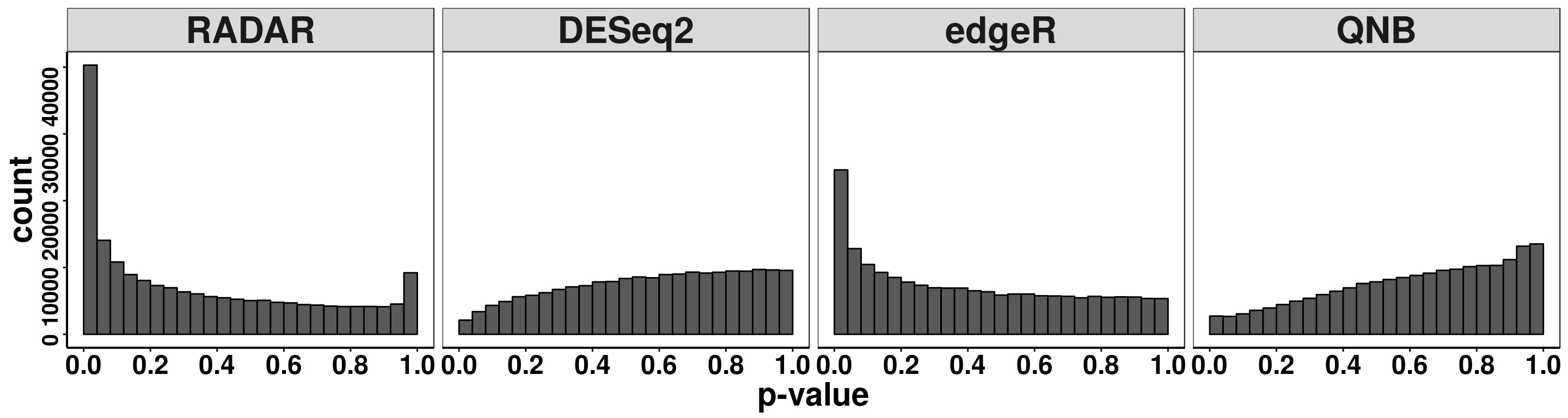

Compare the distibution of beta

par(mfrow = c(1,4))
hist(RADAR$all.est[,"beta1"],main = "RADAR",xlab = "beta",breaks = 50,col =rgb(0.2,0.2,0.2,0.5),cex.main = 2.5,cex.axis =2,cex.lab=2)
hist(deseq2.res$log2FC, main = "DESeq2",xlab = "beta",breaks = 100,col =rgb(0.2,0.2,0.2,0.5),cex.main = 2.5,cex.axis =2,cex.lab=2)
hist(edgeR.res$log2FC,main = "edgeR", xlab = "beta",breaks = 50,col =rgb(0.2,0.2,0.2,0.5),cex.main = 2.5,cex.axis =2,cex.lab=2)
hist(QNB.res$log2.OR, main = "QNB",xlab = "beta",breaks = 50,col =rgb(0.2,0.2,0.2,0.5),cex.main = 2.5,cex.axis =2,cex.lab=2)

Compare norm by geneSum with norm by position

par(mfrow = c(1,3))

tmp <- hist(c(RADAR_pos$all.est[,"p_value3"]),plot = F)
tmp$counts <- tmp$counts*(nrow(RADAR$ip_adjExpr_filtered)/nrow(RADAR_pos$ip_adjExpr_filtered))
hist(RADAR$all.est[,"p_value3"],main = "RADAR",xlab = "p value",col =rgb(1,0,0,0.4),cex.main = 2.5,cex.axis =2,cex.lab=2, ylim = c(0,max(hist(RADAR$all.est[,"p_value3"],plot = F)$counts,tmp$counts)) )
plot(tmp,col=rgb(0,0,1,0.5),add = T)
axis(side = 1, lwd = 1,cex.axis =2)
axis(side = 2, lwd = 1,cex.axis =2)
legend("topright", c("By geneSum", "By position"), col=c(rgb(1,0,0,0.4), rgb(0,0,1,0.5)), lwd = 10,bty="n",text.font = 2)

y.scale <- max(hist(RADAR$all.est[,"p_value3"],plot = F)$counts)

tmp <- hist(c(deseq2.res_pos$pvalue),plot = F)
tmp$counts <- tmp$counts*(nrow(RADAR$ip_adjExpr_filtered)/nrow(RADAR_pos$ip_adjExpr_filtered))
hist(deseq2.res$pvalue,main = "DESeq2",xlab = "p value",col =rgb(1,0,0,0.4),cex.main = 2.5,cex.axis =2,cex.lab=2, ylim = c(0,y.scale) )
plot(tmp,col=rgb(0,0,1,0.5),add = T)
axis(side = 1, lwd = 1,cex.axis =2)
axis(side = 2, lwd = 1,cex.axis =2)
legend("topright", c("By geneSum", "By position"), col=c(rgb(1,0,0,0.4), rgb(0,0,1,0.5)), lwd = 10,bty="n",text.font = 2)

tmp <- hist(c(edgeR.res_pos$pvalue),plot = F)
tmp$counts <- tmp$counts*(nrow(RADAR$ip_adjExpr_filtered)/nrow(RADAR_pos$ip_adjExpr_filtered))
hist(edgeR.res$pvalue,main = "edgeR",xlab = "p value",col =rgb(1,0,0,0.4),cex.main = 2.5,cex.axis =2,cex.lab=2, ylim = c(0,max(hist(edgeR.res$pvalue,plot = F)$counts,tmp$counts,y.scale)) )
plot(tmp,col=rgb(0,0,1,0.5),add = T)
axis(side = 1, lwd = 1,cex.axis =2)
axis(side = 2, lwd = 1,cex.axis =2)
legend("topright", c("By geneSum", "By position"), col=c(rgb(1,0,0,0.4), rgb(0,0,1,0.5)), lwd = 10,bty="n",text.font = 2)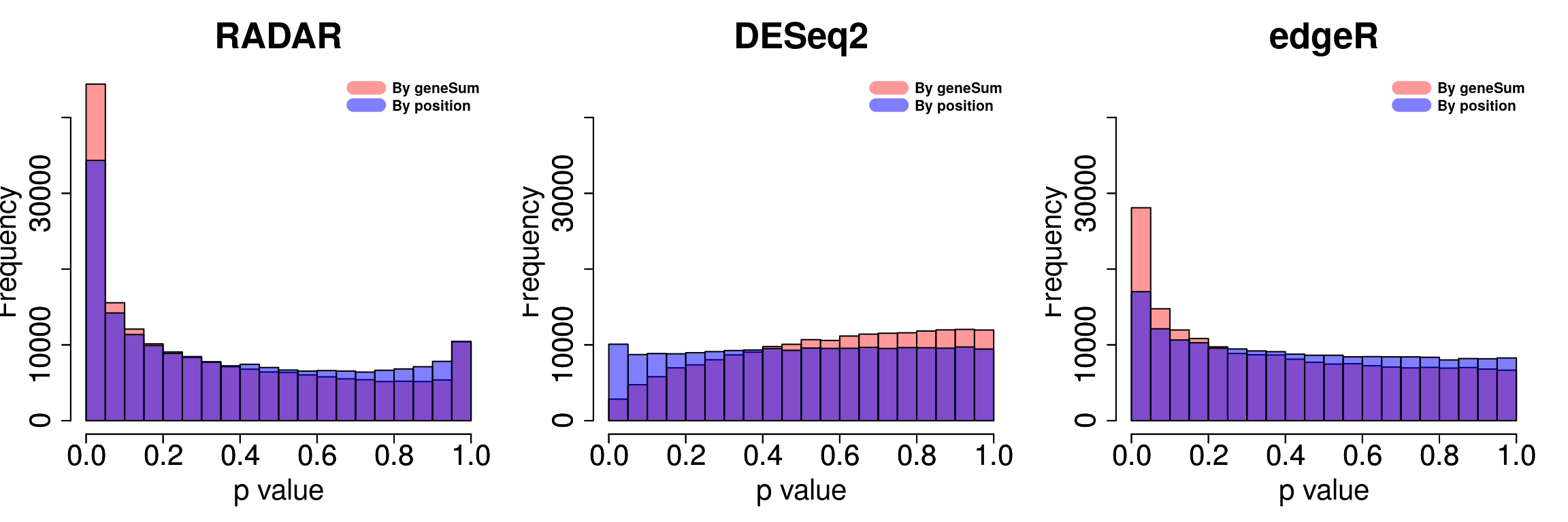

Number of significant bins detected at qvalue < 0.1

sigBins <- apply(cbind("RADAR"=RADAR$all.est[,"p_value3"],"DESeq2"=deseq2.res$pvalue,"edgeR"=edgeR.res$pvalue,"QNB"=QNB.res$pvalue),2, function(x){
  length( which( qvalue::qvalue(x)$qvalue < 0.1 ) )
})
print(sigBins)

##  RADAR DESeq2  edgeR    QNB
##  28031     17   7531     27

Plot overlap of significant hits

plot.new()
MyTools::venn_diagram4( names(which( qvalue::qvalue(RADAR$all.est[,"p_value3"])$qvalue < 0.1 ) ),
                        rownames(RADAR$all.est)[which( qvalue::qvalue(deseq2.res$pvalue)$qvalue < 0.1 ) ],
                        rownames(RADAR$all.est)[which( qvalue::qvalue(edgeR.res$pvalue)$qvalue < 0.1 ) ],
                        rownames(RADAR$all.est)[which( qvalue::qvalue(QNB.res$pvalue)$qvalue < 0.1 ) ],
                        "RADAR","DESeq2","edgeR","QNB")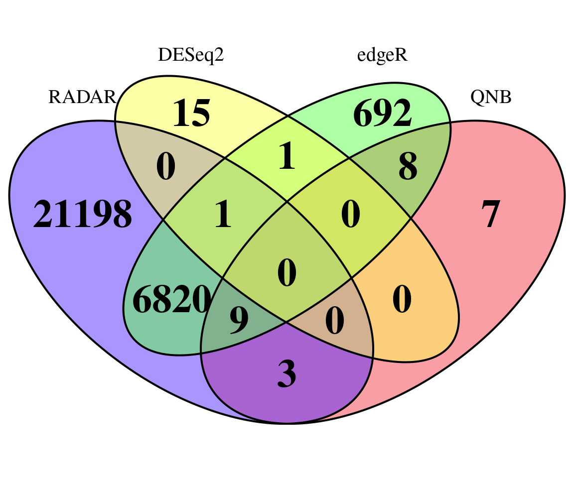

self-FDR test

load("~/PoissonGamma_Method/T2D_data/selfFDR.RData")
ggplot(data = selfFDR, aes(x=method, y= self_FDR, colour = qvalue_cutoff))+geom_boxplot()+theme_bw() +xlab("Method")+ylab("Self-FDR")+ theme(panel.border = element_blank(), panel.grid.major = element_blank(),
                   panel.grid.minor = element_blank(), axis.line = element_line(colour = "black",size = 1),
                   axis.title.x=element_text(size=20, face="bold", hjust=0.5),
                   axis.title.y=element_text(size=20, face="bold", vjust=0.4, angle=90),
                   legend.title=element_text(size = 15,face = "bold"),legend.text = element_text(size = 18, face = "bold",family = "arial"),
                   axis.text = element_text(size = 15,face = "bold",colour = "black") , axis.ticks = element_line(colour = "black",size = 1) )+scale_color_discrete(name = "qvalue\ncutoff")

selfFDR_pos <- NULL
samplenames <- RADAR$samplenames
set.seed(3)
for(i in 1:20){
  ## Sample subset
  sample_id <-  c(sample(x = 1:7, size = 5,replace = F),7+sample(x = 1:8, size = 6,replace = F) )
  Truth_id <- setdiff(1:12,sample_id)


  if(length(unique(X2[sample_id])) == 1 ){ ## samples all from one batch
    ## run radar
  radar_sample <- diffIP_parallel(RADAR_pos[1:14] ,Covariates = cov[,2:3],exclude = samplenames[setdiff(1:15,sample_id)],thread = 15,plotPvalue = F)$all.est
  radar_sample <- cbind(radar_sample, "qvalue"= qvalue::qvalue(radar_sample[,"p_value3"])$qvalue  )
  radar_truth <-  RADAR_pos$all.est
  radar_truth <- cbind(radar_truth, "qvalue"= qvalue::qvalue(radar_truth[,"p_value3"])$qvalue   )

  radar_selfFDR <- sapply(c(0.1,0.05,0.01),function(x){length( which(! which(radar_sample[,"qvalue"]<x) %in% which(radar_truth[,"qvalue"]<0.1) ) )/length(which(radar_sample[,"qvalue"]<x))})

  ## run DESeq2
  deseq_sample <- DESeq2(countdata = RADAR_pos$ip_adjExpr_filtered[,sample_id],pheno = matrix(c(rep(0,7),rep(1,8))[sample_id],ncol = 1),covariates = cov[sample_id,2:3] )
  deseq_sample$qvalue <- qvalue::qvalue( deseq_sample$pvalue )$qvalue
  deseq_truth <- deseq2.res_pos
  deseq_truth$qvalue <- qvalue::qvalue( deseq_truth$pvalue )$qvalue

  deseq_selfFDR <-  sapply(c(0.1,0.05,0.01),function(x){length( which(! which(deseq_sample[,"qvalue"]<x) %in% which(deseq_truth[,"qvalue"]<0.1) ) )/length(which(deseq_sample[,"qvalue"]<x))})

  ## run edgeR
  edgeR_sample <- edgeR(countdata = RADAR_pos$ip_adjExpr_filtered[,sample_id],pheno = matrix(c(rep(0,7),rep(1,8))[sample_id],ncol = 1),covariates = cov[sample_id,2:3] )
  edgeR_sample$qvalue <- qvalue::qvalue( edgeR_sample$pvalue )$qvalue
  edgeR_truth <- edgeR.res_pos
  edgeR_truth$qvalue <- qvalue::qvalue( edgeR_truth$pvalue )$qvalue

  edgeR_selfFDR <-  sapply(c(0.1,0.05,0.01),function(x){length( which(! which(edgeR_sample[,"qvalue"]<x) %in% which(edgeR_truth[,"qvalue"]<0.1) ) )/length(which(edgeR_sample[,"qvalue"]<x))})

   fdr <- rbind( data.frame(self_FDR = radar_selfFDR, qvalue_cutoff=c("0.1","0.05","0.01"), method = rep("RADAR",3) ),
                   data.frame(self_FDR = deseq_selfFDR, qvalue_cutoff=c("0.1","0.05","0.01"), method = rep("DESeq2",3) ),
                   data.frame(self_FDR = edgeR_selfFDR, qvalue_cutoff=c("0.1","0.05","0.01"), method = rep("edgeR",3) )
                   )

  selfFDR_pos <- rbind(selfFDR_pos,fdr)
  }else if(length(unique(X3[sample_id])) == 1 ){
     ## run radar
  radar_sample <- diffIP_parallel(RADAR_pos[1:14] ,Covariates = cov[,c(1,3)],exclude = samplenames[setdiff(1:15,sample_id)],thread = 15,plotPvalue = F)$all.est
  radar_sample <- cbind(radar_sample, "qvalue"= qvalue::qvalue(radar_sample[,"p_value3"])$qvalue  )
  radar_truth <-  RADAR_pos$all.est
  radar_truth <- cbind(radar_truth, "qvalue"= qvalue::qvalue(radar_truth[,"p_value3"])$qvalue   )

  radar_selfFDR <- sapply(c(0.1,0.05,0.01),function(x){length( which(! which(radar_sample[,"qvalue"]<x) %in% which(radar_truth[,"qvalue"]<0.1) ) )/length(which(radar_sample[,"qvalue"]<x))})

  ## run DESeq2
  deseq_sample <- DESeq2(countdata = RADAR_pos$ip_adjExpr_filtered[,sample_id],pheno = matrix(c(rep(0,7),rep(1,8))[sample_id],ncol = 1),covariates = cov[sample_id,c(1,3)] )
  deseq_sample$qvalue <- qvalue::qvalue( deseq_sample$pvalue )$qvalue
  deseq_truth <- deseq2.res_pos
  deseq_truth$qvalue <- qvalue::qvalue( deseq_truth$pvalue )$qvalue

  deseq_selfFDR <-  sapply(c(0.1,0.05,0.01),function(x){length( which(! which(deseq_sample[,"qvalue"]<x) %in% which(deseq_truth[,"qvalue"]<0.1) ) )/length(which(deseq_sample[,"qvalue"]<x))})

  ## run edgeR
  edgeR_sample <- edgeR(countdata = RADAR_pos$ip_adjExpr_filtered[,sample_id],pheno = matrix(c(rep(0,7),rep(1,8))[sample_id],ncol = 1),covariates = cov[sample_id,c(1,3)] )
  edgeR_sample$qvalue <- qvalue::qvalue( edgeR_sample$pvalue )$qvalue
  edgeR_truth <- edgeR.res_pos
  edgeR_truth$qvalue <- qvalue::qvalue( edgeR_truth$pvalue )$qvalue

   edgeR_selfFDR <-  sapply(c(0.1,0.05,0.01),function(x){length( which(! which(edgeR_sample[,"qvalue"]<x) %in% which(edgeR_truth[,"qvalue"]<0.1) ) )/length(which(edgeR_sample[,"qvalue"]<x))})

   fdr <- rbind( data.frame(self_FDR = radar_selfFDR, qvalue_cutoff=c("0.1","0.05","0.01"), method = rep("RADAR",3) ),
                   data.frame(self_FDR = deseq_selfFDR, qvalue_cutoff=c("0.1","0.05","0.01"), method = rep("DESeq2",3) ),
                   data.frame(self_FDR = edgeR_selfFDR, qvalue_cutoff=c("0.1","0.05","0.01"), method = rep("edgeR",3) )
                   )

  selfFDR_pos <- rbind(selfFDR_pos,fdr)
  }else if(length(unique(X4[sample_id])) == 1){
  ## run radar
  radar_sample <- diffIP_parallel(RADAR_pos[1:14] ,Covariates = cov[,c(1,2)],exclude = samplenames[setdiff(1:15,sample_id)],thread = 15,plotPvalue = F)$all.est
  radar_sample <- cbind(radar_sample, "qvalue"= qvalue::qvalue(radar_sample[,"p_value3"])$qvalue  )
  radar_truth <-  RADAR_pos$all.est
  radar_truth <- cbind(radar_truth, "qvalue"= qvalue::qvalue(radar_truth[,"p_value3"])$qvalue   )

  radar_selfFDR <- sapply(c(0.1,0.05,0.01),function(x){length( which(! which(radar_sample[,"qvalue"]<x) %in% which(radar_truth[,"qvalue"]<0.1) ) )/length(which(radar_sample[,"qvalue"]<x))})

  ## run DESeq2
  deseq_sample <- DESeq2(countdata = RADAR_pos$ip_adjExpr_filtered[,sample_id],pheno = matrix(c(rep(0,7),rep(1,8))[sample_id],ncol = 1),covariates = cov[sample_id,c(1,2)] )
  deseq_sample$qvalue <- qvalue::qvalue( deseq_sample$pvalue )$qvalue
  deseq_truth <- deseq2.res_pos
  deseq_truth$qvalue <- qvalue::qvalue( deseq_truth$pvalue )$qvalue

  deseq_selfFDR <-  sapply(c(0.1,0.05,0.01),function(x){length( which(! which(deseq_sample[,"qvalue"]<x) %in% which(deseq_truth[,"qvalue"]<0.1) ) )/length(which(deseq_sample[,"qvalue"]<x))})

  ## run edgeR
  edgeR_sample <- edgeR(countdata = RADAR_pos$ip_adjExpr_filtered[,sample_id],pheno = matrix(c(rep(0,7),rep(1,8))[sample_id],ncol = 1),covariates = cov[sample_id,c(1,2)] )
  edgeR_sample$qvalue <- qvalue::qvalue( edgeR_sample$pvalue )$qvalue
  edgeR_truth <- edgeR.res_pos
  edgeR_truth$qvalue <- qvalue::qvalue( edgeR_truth$pvalue )$qvalue

   edgeR_selfFDR <-  sapply(c(0.1,0.05,0.01),function(x){length( which(! which(edgeR_sample[,"qvalue"]<x) %in% which(edgeR_truth[,"qvalue"]<0.1) ) )/length(which(edgeR_sample[,"qvalue"]<x))})

   fdr <- rbind( data.frame(self_FDR = radar_selfFDR, qvalue_cuttoff=c("0.1","0.05","0.01"), method = rep("RADAR",3) ),
                   data.frame(self_FDR = deseq_selfFDR, qvalue_cuttoff=c("0.1","0.05","0.01"), method = rep("DESeq2",3) ),
                   data.frame(self_FDR = edgeR_selfFDR, qvalue_cuttoff=c("0.1","0.05","0.01"), method = rep("edgeR",3) )
                   )

  selfFDR_pos <- rbind(selfFDR_pos,fdr)
  }else{
  ## run radar
  radar_sample <- diffIP_parallel(RADAR_pos[1:14],Covariates = cov ,exclude = samplenames[setdiff(1:15,sample_id)],thread = 15,plotPvalue = F)$all.est
  radar_sample <- cbind(radar_sample, "qvalue"= qvalue::qvalue(radar_sample[,"p_value3"])$qvalue  )
  radar_truth <-  RADAR_pos$all.est
  radar_truth <- cbind(radar_truth, "qvalue"= qvalue::qvalue(radar_truth[,"p_value3"])$qvalue   )

  radar_selfFDR <- sapply(c(0.1,0.05,0.01),function(x){length( which(! which(radar_sample[,"qvalue"]<x) %in% which(radar_truth[,"qvalue"]<0.1) ) )/length(which(radar_sample[,"qvalue"]<x))})

  ## run DESeq2
  deseq_sample <- DESeq2(countdata = RADAR_pos$ip_adjExpr_filtered[,sample_id],pheno = matrix(c(rep(0,7),rep(1,8))[sample_id],ncol = 1),covariates =  cov[sample_id,] )
  deseq_sample$qvalue <- qvalue::qvalue( deseq_sample$pvalue )$qvalue
  deseq_truth <- deseq2.res_pos
  deseq_truth$qvalue <- qvalue::qvalue( deseq_truth$pvalue )$qvalue

  deseq_selfFDR <-  sapply(c(0.1,0.05,0.01),function(x){length( which(! which(deseq_sample[,"qvalue"]<x) %in% which(deseq_truth[,"qvalue"]<0.1) ) )/length(which(deseq_sample[,"qvalue"]<x))})

  ## run edgeR
  edgeR_sample <- edgeR(countdata = RADAR_pos$ip_adjExpr_filtered[,sample_id],pheno = matrix(c(rep(0,7),rep(1,8))[sample_id],ncol = 1),covariates =  cov[sample_id,] )
  edgeR_sample$qvalue <- qvalue::qvalue( edgeR_sample$pvalue )$qvalue
  edgeR_truth <- edgeR.res_pos
  edgeR_truth$qvalue <- qvalue::qvalue( edgeR_truth$pvalue )$qvalue

   edgeR_selfFDR <-  sapply(c(0.1,0.05,0.01),function(x){length( which(! which(edgeR_sample[,"qvalue"]<x) %in% which(edgeR_truth[,"qvalue"]<0.1) ) )/length(which(edgeR_sample[,"qvalue"]<x))})

   fdr <- rbind( data.frame(self_FDR = radar_selfFDR, qvalue_cutoff=c("0.1","0.05","0.01"), method = rep("RADAR",3) ),
                   data.frame(self_FDR = deseq_selfFDR, qvalue_cutoff=c("0.1","0.05","0.01"), method = rep("DESeq2",3) ),
                   data.frame(self_FDR = edgeR_selfFDR, qvalue_cutoff=c("0.1","0.05","0.01"), method = rep("edgeR",3) )
                   )

  selfFDR_pos <- rbind(selfFDR_pos,fdr)
  }
}
selfFDR_pos$qvalue_cutoff <- factor(selfFDR_pos$qvalue_cutoff,levels = c("0.1","0.05","0.01"))
save(selfFDR_pos, file = "~/PoissonGamma_Method/T2D_data/selfFDR_pos.RData")

Self-FDR norm by local bin read count

load("~/PoissonGamma_Method/T2D_data/selfFDR_pos.RData")
selfFDR_all <- cbind(rbind(selfFDR, selfFDR_pos), "NormBy"= c(rep("By gene-level count",nrow(selfFDR)),rep("By bin-level count",nrow(selfFDR_pos))) )
selfFDR_all$NormBy <- factor(selfFDR_all$NormBy,levels = c("By gene-level count","By bin-level count"))

ggplot(data = selfFDR_all, aes(x=method, y= self_FDR, colour = qvalue_cutoff))+geom_boxplot()+facet_grid(~NormBy)+theme_bw()  +xlab("Method")+ylab("Self-FDR")+ theme( panel.grid.major = element_blank(),
                   axis.line = element_line(colour = "black",size = 1),
                   axis.title.x=element_text(size=20, face="bold", hjust=0.5,family = "arial"),
                   axis.title.y=element_text(size=20, face="bold", vjust=0.4, angle=90,family = "arial"),
                   legend.title=element_text(size = 15,face = "bold"),legend.text = element_text(size = 18, face = "bold",family = "arial"),
                   axis.text = element_text(size = 18,face = "bold",family = "arial",colour = "black") ,strip.text.x = element_text(size = 20,face = "bold") )+scale_color_discrete(name = "qvalue\ncutoff")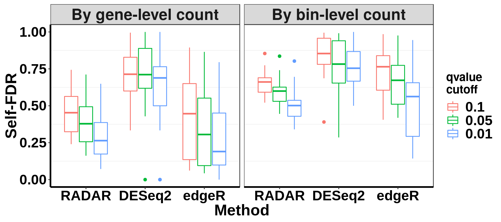

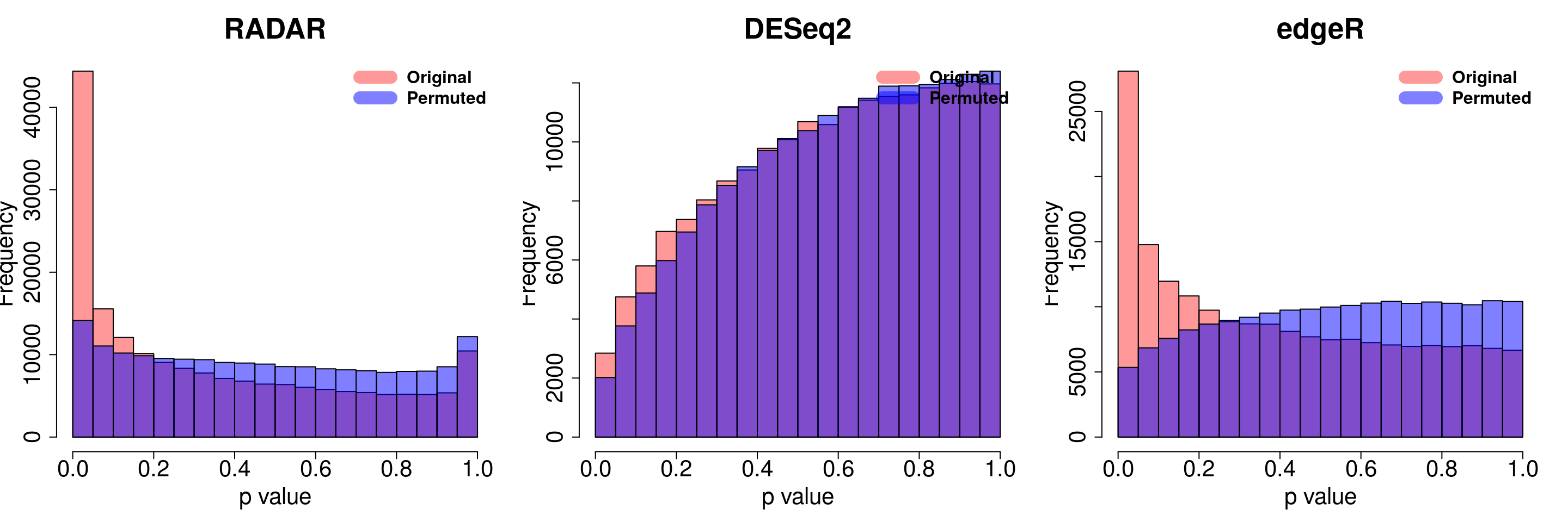
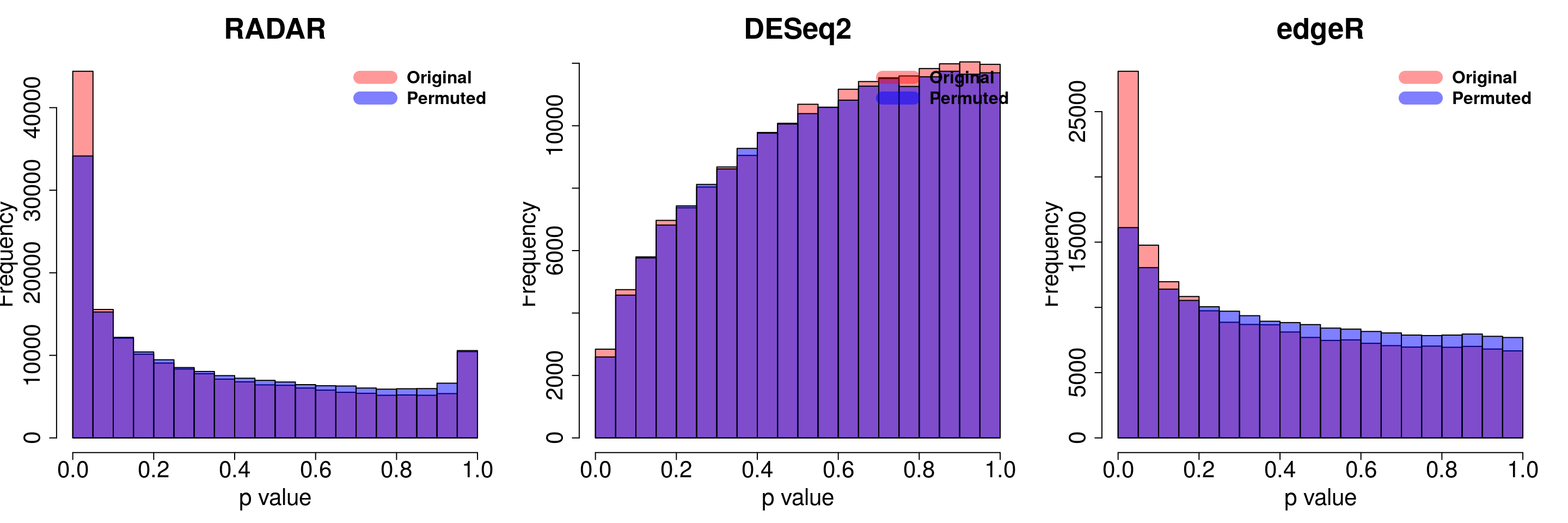
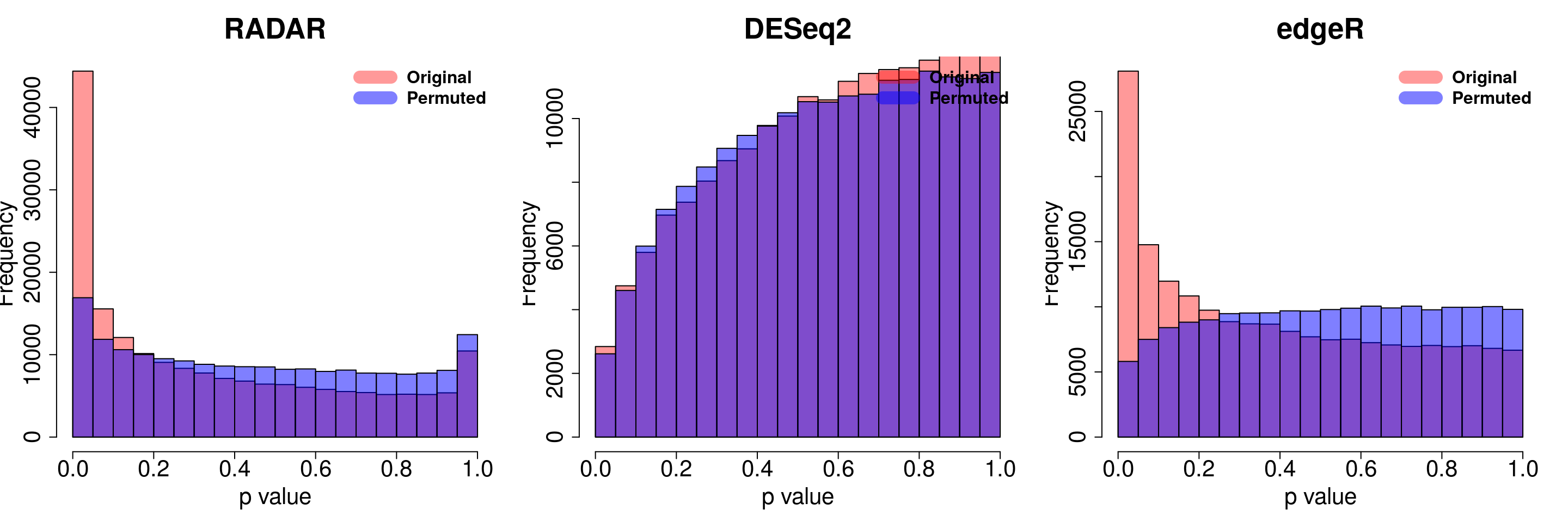
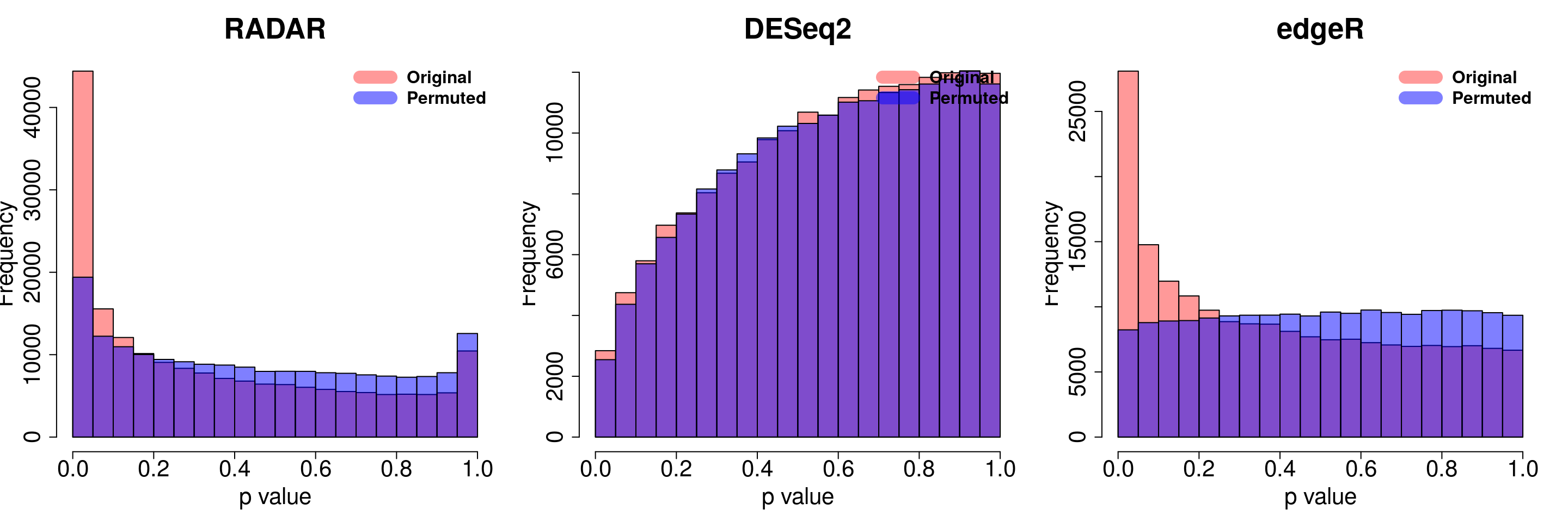
Permution

radar_permuted_P <-NULL
deseq_permuted_P <- NULL
edgeR_permuted_P <- NULL

set.seed(51)
for(i in 1:10){

  permute_X <- unlist( tapply(RADAR$X,batch,function(x){sample(x,length(x))}) )[match(RADAR$samplenames,unlist( tapply(RADAR$samplenames,batch,function(x)return(x)) ))]
  if ( all( permute_X == RADAR$X) | all( permute_X == c(rep("T2D",8),rep("Ctl",7))) ){
    cat("Duplicated with original design...\n")
  }else{
    radar_permute <- diffIP_parallel(c(RADAR[1:11],list("X"=permute_X),RADAR[13:14]) ,thread = 15,Covariates = cov,plotPvalue = F)$all.est[,"p_value3"]
    deseq_permute <- DESeq2(countdata = RADAR$ip_adjExpr_filtered,pheno = matrix(permute_X,ncol = 1),covariates = cov )$pvalue
    edgeR_permute <- edgeR(countdata = RADAR$ip_adjExpr_filtered,pheno = matrix(permute_X,ncol = 1),covariates =  cov )$pvalue

    radar_permuted_P <- cbind(radar_permuted_P, radar_permute)
    deseq_permuted_P <- cbind(deseq_permuted_P,deseq_permute)
    edgeR_permuted_P <- cbind(edgeR_permuted_P,edgeR_permute)
  }
}
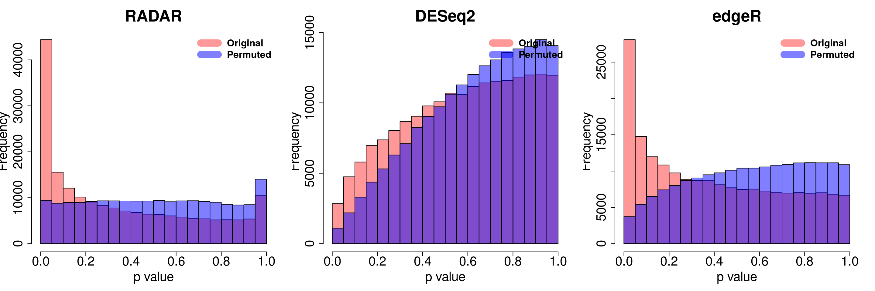
save(radar_permuted_P ,deseq_permuted_P ,edgeR_permuted_P, file= "~/PoissonGamma_Method/T2D_data/permutation.RData")

load( "~/PoissonGamma_Method/T2D_data/permutation.RData")
for( i in 1:ncol(radar_permuted_P)){
par(mfrow=c(1,3))
hist(RADAR$all.est[,"p_value3"], col =rgb(1,0,0,0.4),main = "RADAR", xlab = "p value",cex.main = 2.5,cex.axis =2,cex.lab=2)
hist(radar_permuted_P[,i],col=rgb(0,0,1,0.5),add = T)
legend("topright", c("Original", "Permuted"), col=c(rgb(1,0,0,0.4), rgb(0,0,1,0.5)), lwd = 12,bty="n",text.font = 2, cex = 1.5)

hist(deseq2.res$pvalue, col =rgb(1,0,0,0.4),main = "DESeq2",xlab = "p value",cex.main = 2.5,cex.axis =2,cex.lab=2, ylim =c(0,max(hist(deseq_permuted_P[,i],plot = F)$counts) ) )
hist(deseq_permuted_P[,i],col=rgb(0,0,1,0.5),add = T)
legend("topright", c("Original", "Permuted"), col=c(rgb(1,0,0,0.4), rgb(0,0,1,0.5)), lwd = 12,bty="n",text.font = 2, cex = 1.5)

hist(edgeR.res$pvalue, col =rgb(1,0,0,0.4),main = "edgeR",xlab = "p value",cex.main = 2.5,cex.axis =2,cex.lab=2)
hist(edgeR_permuted_P[,i],col=rgb(0,0,1,0.5),add = T)
legend("topright", c("Original", "Permuted"), col=c(rgb(1,0,0,0.4), rgb(0,0,1,0.5)), lwd = 12,bty="n",text.font = 2, cex = 1.5)

}

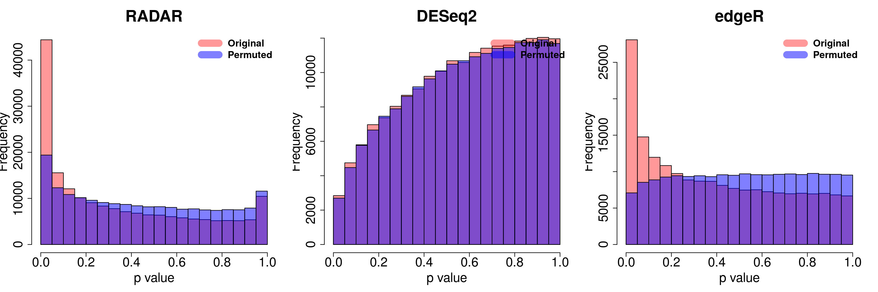
combine all sets of permuted p value in one

par(mfrow=c(1,2))
hist(RADAR$all.est[,"p_value3"], col =rgb(1,0,0,0.4),main = "RADAR", xlab = "p value",font=2, cex.lab=1.5,  font.lab=2 ,cex.main = 2,cex.axis =1, lwd = 2.5)
tmp <- hist(c(radar_permuted_P),plot = F)
tmp$counts <- tmp$counts/10
plot(tmp,col=rgb(0,0,1,0.5),add = T)
legend("topright", c("Original", "Permuted"), col=c(rgb(1,0,0,0.4), rgb(0,0,1,0.5)), lwd = 12,bty="n",text.font = 2, cex = 1)

y.scale <- max(hist(RADAR$all.est[,"p_value3"],plot = F)$counts)

#hist(deseq2.res$pvalue, col =rgb(1,0,0,0.4),main = "DESeq2",xlab = "p value")
#tmp <- hist(c(deseq_permuted_P),plot = F)
#tmp$counts <- tmp$counts/10
#plot(tmp,col=rgb(0,0,1,0.5),add = T)
#legend("topright", c("Original", "Permuted"), col=c(rgb(1,0,0,0.4), rgb(0,0,1,0.5)), lwd = 10,bty="n")
hist(edgeR.res$pvalue, col =rgb(1,0,0,0.4),main = "edgeR",xlab = "p value",font=2, cex.lab=1.5,  font.lab=2 ,cex.main = 2 , cex.axis =1, ylim = c(0,y.scale), lwd = 2.5)
tmp <- hist(c(edgeR_permuted_P),plot = F)
tmp$counts <- tmp$counts/10
plot(tmp,col=rgb(0,0,1,0.5),add = T)
legend("topright", c("Original", "Permuted"), col=c(rgb(1,0,0,0.4), rgb(0,0,1,0.5)), lwd = 12,bty="n",text.font = 2, cex = 1)

Plot Heat map of significant bins by RADAR

topBins <- RADAR$ip_adjExpr_filtered[which(qvalue(RADAR$all.est[,"p_value3"])$qvalue<0.1),]
log_topBins <- log(topBins+1)

    registerDoParallel(cores = 4)
    cov.out.RADAR <- foreach(i = 1:nrow(log_topBins), .combine = rbind) %dopar% {
      Y = log_topBins[i,]
      tmp_data <- as.data.frame(cbind(Y,cov))
      resi <- residuals( lm(Y~.,data=tmp_data  ) )
      resi
    }
    rm(list=ls(name=foreach:::.foreachGlobals), pos=foreach:::.foreachGlobals)
    rownames(cov.out.RADAR) <- rownames(log_topBins)
    colnames(cov.out.RADAR) <- colnames(log_topBins)

    dist.pear <- function(x) as.dist(1-cor(t(x)))
    hclust.ave <- function(x) hclust(x, method="average")
    gplots::heatmap.2(cov.out.RADAR,scale="row",trace="none",labRow=NA,main = "Methylation level of significant bins\n(Covariates regressed out)",
                      distfun=dist.pear, hclustfun=hclust.ave,col=rev(RColorBrewer::brewer.pal(9,"RdBu")))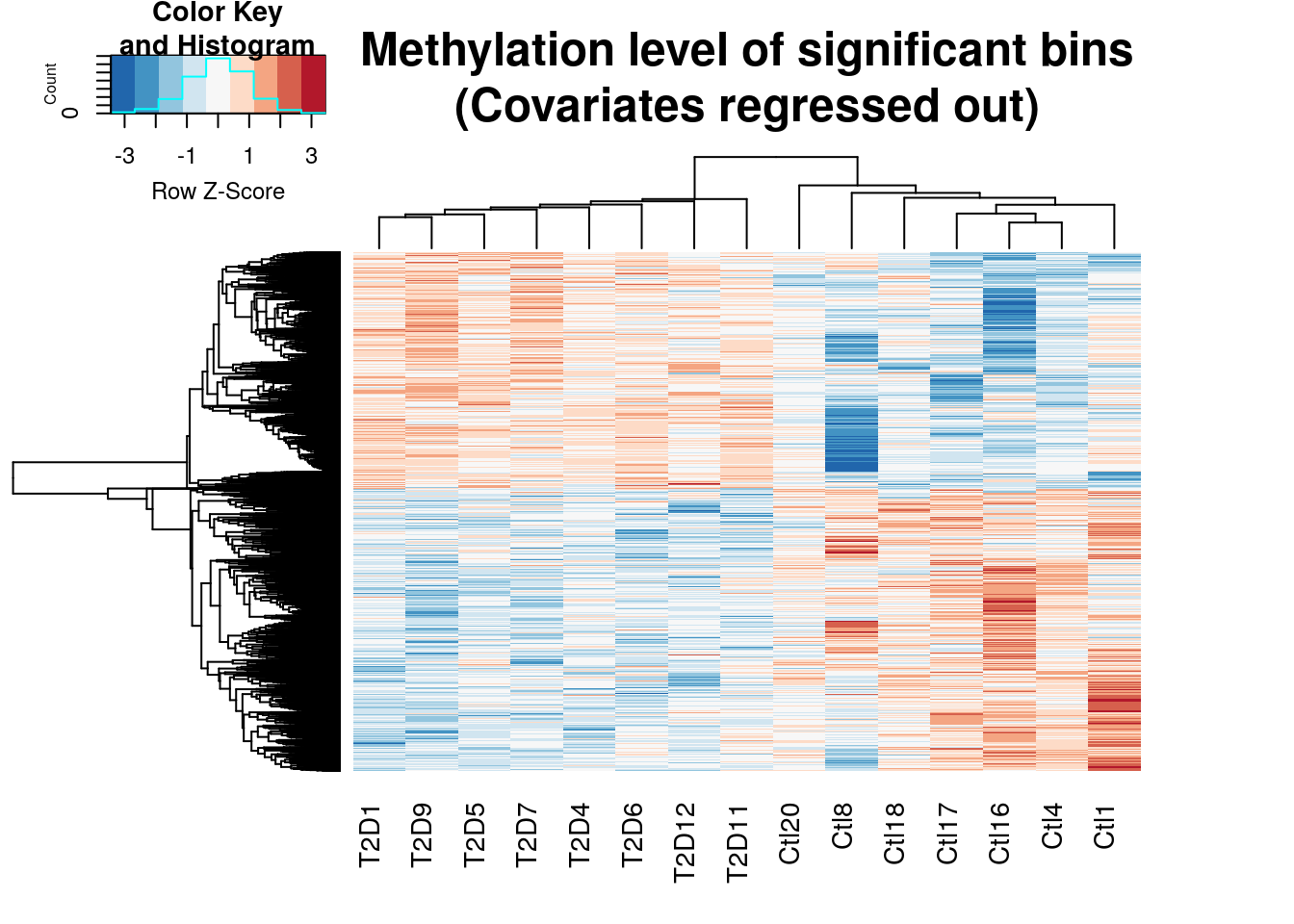

Plot heap map of significant bins by edgeR

topBins <- RADAR$ip_adjExpr_filtered[which(qvalue(edgeR.res$pvalue)$qvalue<0.1),]
log_topBins <- log(topBins+1)

    registerDoParallel(cores = 4)
    cov.out.edgeR <- foreach(i = 1:nrow(log_topBins), .combine = rbind) %dopar% {
      Y = log_topBins[i,]
      tmp_data <- as.data.frame(cbind(Y,cov))
      resi <- residuals( lm(Y~.,data=tmp_data  ) )
      resi
    }
    rm(list=ls(name=foreach:::.foreachGlobals), pos=foreach:::.foreachGlobals)
    rownames(cov.out.edgeR) <- rownames(log_topBins)
    colnames(cov.out.edgeR) <- colnames(log_topBins)

    dist.pear <- function(x) as.dist(1-cor(t(x)))
    hclust.ave <- function(x) hclust(x, method="average")
    gplots::heatmap.2(cov.out.edgeR,scale="row",trace="none",labRow=NA,main = "Methylation level of significant bins\n(Covariates regressed out)",
                      distfun=dist.pear, hclustfun=hclust.ave,col=rev(RColorBrewer::brewer.pal(9,"RdBu")))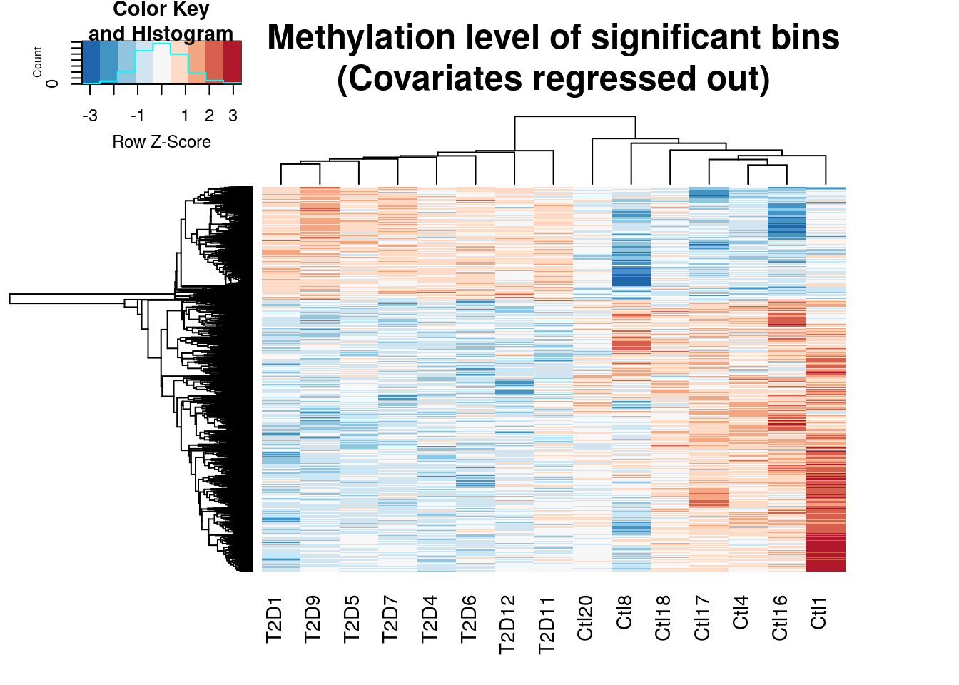

Session information

sessionInfo()

## R version 3.4.4 (2018-03-15)
## Platform: x86_64-pc-linux-gnu (64-bit)
## Running under: Ubuntu 17.10
##
## Matrix products: default
## BLAS: /usr/local/lib/R/lib/libRblas.so
## LAPACK: /usr/local/lib/R/lib/libRlapack.so
##
## locale:
##  [1] LC_CTYPE=en_US.UTF-8       LC_NUMERIC=C
##  [3] LC_TIME=en_US.UTF-8        LC_COLLATE=en_US.UTF-8
##  [5] LC_MONETARY=en_US.UTF-8    LC_MESSAGES=en_US.UTF-8
##  [7] LC_PAPER=en_US.UTF-8       LC_NAME=C
##  [9] LC_ADDRESS=C               LC_TELEPHONE=C
## [11] LC_MEASUREMENT=en_US.UTF-8 LC_IDENTIFICATION=C
##
## attached base packages:
##  [1] grid      stats4    parallel  stats     graphics  grDevices utils
##  [8] datasets  methods   base
##
## other attached packages:
##  [1] VennDiagram_1.6.20        futile.logger_1.4.3
##  [3] qvalue_2.10.0             RADAR_0.1.5
##  [5] RcppArmadillo_0.9.100.5.0 Rcpp_0.12.19
##  [7] RColorBrewer_1.1-2        gplots_3.0.1
##  [9] doParallel_1.0.14         iterators_1.0.10
## [11] foreach_1.4.4             ggplot2_3.0.0
## [13] Rsamtools_1.30.0          Biostrings_2.46.0
## [15] XVector_0.18.0            GenomicFeatures_1.30.3
## [17] AnnotationDbi_1.40.0      Biobase_2.38.0
## [19] GenomicRanges_1.30.3      GenomeInfoDb_1.14.0
## [21] IRanges_2.12.0            S4Vectors_0.16.0
## [23] BiocGenerics_0.24.0
##
## loaded via a namespace (and not attached):
##  [1] nlme_3.1-131.1             bitops_1.0-6
##  [3] matrixStats_0.54.0         bit64_0.9-7
##  [5] progress_1.2.0             httr_1.3.1
##  [7] rprojroot_1.3-2            tools_3.4.4
##  [9] backports_1.1.2            R6_2.2.2
## [11] KernSmooth_2.23-15         mgcv_1.8-23
## [13] DBI_1.0.0                  lazyeval_0.2.1
## [15] colorspace_1.3-2           withr_2.1.2
## [17] gridExtra_2.3              tidyselect_0.2.4
## [19] prettyunits_1.0.2          RMySQL_0.10.15
## [21] bit_1.1-14                 compiler_3.4.4
## [23] formatR_1.5                DelayedArray_0.4.1
## [25] labeling_0.3               rtracklayer_1.38.3
## [27] caTools_1.17.1             scales_0.5.0
## [29] stringr_1.3.1              digest_0.6.15
## [31] rmarkdown_1.10             DOSE_3.4.0
## [33] pkgconfig_2.0.1            htmltools_0.3.6
## [35] highr_0.7                  rlang_0.2.1
## [37] RSQLite_2.1.1              bindr_0.1.1
## [39] BiocParallel_1.12.0        gtools_3.8.1
## [41] GOSemSim_2.4.1             dplyr_0.7.6
## [43] RCurl_1.95-4.10            magrittr_1.5
## [45] GO.db_3.5.0                GenomeInfoDbData_1.0.0
## [47] Matrix_1.2-12              munsell_0.5.0
## [49] stringi_1.2.3              yaml_2.1.19
## [51] SummarizedExperiment_1.8.1 zlibbioc_1.24.0
## [53] plyr_1.8.4                 blob_1.1.1
## [55] gdata_2.18.0               DO.db_2.9
## [57] crayon_1.3.4               lattice_0.20-35
## [59] splines_3.4.4              hms_0.4.2
## [61] knitr_1.20                 pillar_1.2.3
## [63] igraph_1.2.1               fgsea_1.4.1
## [65] reshape2_1.4.3             codetools_0.2-15
## [67] biomaRt_2.34.2             futile.options_1.0.1
## [69] fastmatch_1.1-0            XML_3.98-1.11
## [71] glue_1.2.0                 evaluate_0.10.1
## [73] lambda.r_1.2.3             data.table_1.11.4
## [75] tidyr_0.8.1                gtable_0.2.0
## [77] purrr_0.2.5                assertthat_0.2.0
## [79] tibble_1.4.2               clusterProfiler_3.6.0
## [81] rvcheck_0.1.0              GenomicAlignments_1.14.2
## [83] memoise_1.1.0              MyTools_0.0.0
## [85] bindrcpp_0.2.2

This R Markdown site was created with workflowr

T2D

Zijie Zhang

2018-08-21