MouseLiver

Count reads

library(RADAR)

samplenames = c("4582WT","4584WT","4587WT","4612WT","4583KO","4586KO","4615KO","4616KO")

RADAR <- countReads(samplenames = samplenames,
                  gtf = "/home/zijiezhang/Database/genome/mm10/mm10_UCSC.gtf",
                  bamFolder = "~/METTL14_liver2017/bam_files/",
                  outputDir = "~/METTL14/RADAR",
                  modification = "m6A",
                  threads = 8
)

Summary of read count

library(RADAR)
#load("~/METTL14_liver2017/RDM.RData")
load("~/PoissonGamma_Method/M14liver/RADAR_analysis.RData")
countSummary <- rbind("Input"= colSums(RADAR$reads)[1:length(RADAR$samplenames)], "IP" =colSums(RADAR$reads)[(1:length(RADAR$samplenames))+length(RADAR$samplenames)] )
colnames(countSummary) <- RADAR$samplenames
knitr::kable(countSummary,format = "pandoc" )

	4582WT	4584WT	4587WT	4612WT	4583KO	4586KO	4615KO	4616KO
Input	19226065	16782163	16613239	17355731	22416046	17879630	17243007	18956379
IP	18794825	21706060	19979393	20282034	19224643	21704815	20873547	18258523

X <- c(rep("WT",4),rep("KO",4))
RADAR <- normalizeLibrary(RADAR,X)
RADAR <- RADAR::adjustExprLevel(RADAR)
RADAR <- filterBins(RADAR,minCountsCutOff = 15)

Plot distribution of number of reads in each 50 bp bins

hist(log10(rowMeans(RADAR$reads[rowMeans(RADAR$reads[,grep("input",colnames(RADAR$reads))])>1,grep("input",colnames(RADAR$reads))])  ),xlab = "log10 read count",main = "Distribution of INPUT read count in bins",xlim = c(0,3), col =rgb(0.2,0.2,0.2,0.5),cex.main = 2,cex.axis =2,cex.lab=2)
axis(side = 1, lwd = 2,cex.axis =2)
axis(side = 2, lwd = 2,cex.axis =2)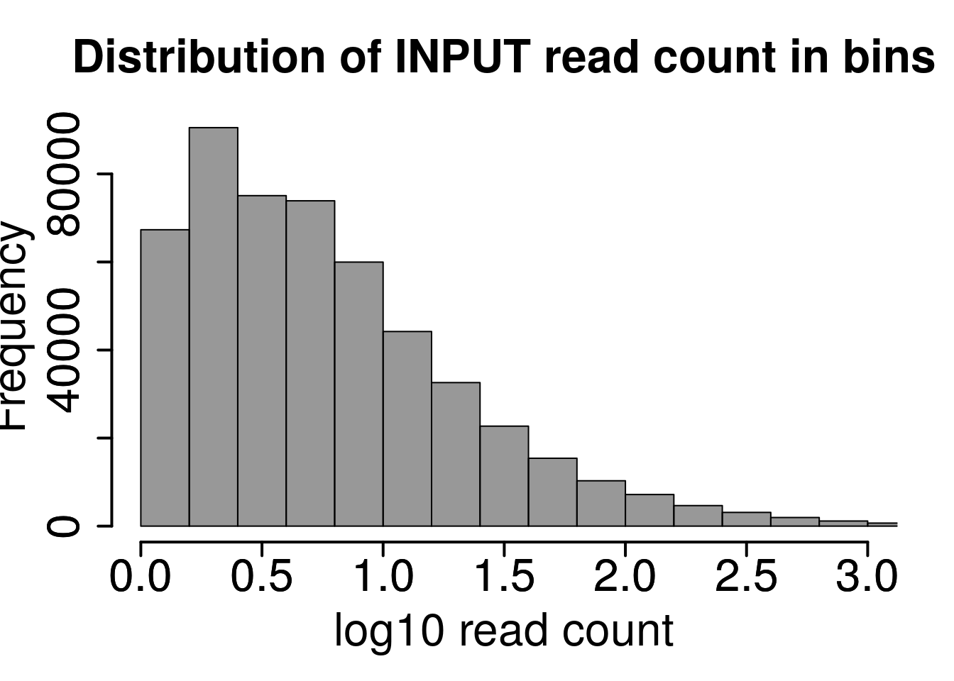

local read count V.S. geneSum

Compute the within group variability of INPUT geneSum VS INPUT local read count.

var.coef <- function(x){sd(as.numeric(x))/mean(as.numeric(x))}
## filter expressed genes
geneSum <- RADAR$geneSum[rowSums(RADAR$geneSum)>16,]
## within group variability
relative.var <- t( apply(geneSum,1,tapply,RADAR$X,var.coef) )
geneSum.var <- c(relative.var)

## For each gene used above, random sample a 50bp bin within this gene
set.seed(1)
r.bin50 <- tapply(rownames(RADAR$norm.input)[which(RADAR$geneBins$gene %in% rownames(geneSum))],as.character( RADAR$geneBins$gene[which(RADAR$geneBins$gene %in% rownames(geneSum))]) ,function(x){
  n <- sample(1:length(x),1)
  return(x[n])
})

relative.var <- apply(RADAR$norm.input[r.bin50,],1,tapply,RADAR$X,var.coef)
bin50.var <- c(relative.var)
bin50.var <- bin50.var[!is.na(bin50.var)]

## 100bp bins
r.bin100 <- tapply(rownames(RADAR$norm.input)[which(RADAR$geneBins$gene %in% rownames(geneSum))],as.character( RADAR$geneBins$gene[which(RADAR$geneBins$gene %in% rownames(geneSum))]) ,function(x){
  n <- sample(1:(length(x)-2),1)
  return(x[n:(n+1)])
})
relative.var <- lapply(r.bin100, function(x){ tapply( colSums(RADAR$norm.input[x,]),RADAR$X,var.coef ) })
bin100.var <- unlist(relative.var)
bin100.var <- bin100.var[!is.na(bin100.var)]

## 200bp bins
r.bin200 <- tapply(rownames(RADAR$norm.input)[which(RADAR$geneBins$gene %in% rownames(geneSum))],as.character( RADAR$geneBins$gene[which(RADAR$geneBins$gene %in% rownames(geneSum))]) ,function(x){
  if(length(x)>4){
    n <- sample(1:(length(x)-3),1)
    return(x[n:(n+3)])
  }else{
    return(NULL)
  }
})
r.bin200 <- r.bin200[which(!unlist(lapply(r.bin200,is.null)) ) ]
relative.var <- lapply(r.bin200, function(x){ tapply( colSums(RADAR$norm.input[x,]),RADAR$X,var.coef ) })

bin200.var <- unlist(relative.var)
bin200.var <- bin200.var[!is.na(bin200.var)]

relative.var <- data.frame(group=c(rep("geneSum",length(geneSum.var)),rep("bin-50bp",length(bin50.var)),rep("bin-100bp",length(bin100.var)),rep("bin-200bp",length(bin200.var))), variance=c(geneSum.var,bin50.var,bin100.var,bin200.var))

ggplot(relative.var,aes(variance,colour=group))+geom_density()+xlab("Relative variation")+
  theme_bw() + theme(panel.border = element_blank(), panel.grid.major = element_blank(),
                   panel.grid.minor = element_blank(), axis.line = element_line(colour = "black",size = 1),
                   axis.title.x=element_text(size=20, face="bold", hjust=0.5,family = "arial"),
                   axis.title.y=element_text(size=20, face="bold", vjust=0.4, angle=90,family = "arial"),
                   legend.position = c(0.88,0.88),legend.title=element_blank(),legend.text = element_text(size = 14, face = "bold",family = "arial"),
                   axis.text.x = element_text(size = 15,face = "bold",family = "arial") ,axis.text.y = element_text(size = 15,face = "bold",family = "arial")  )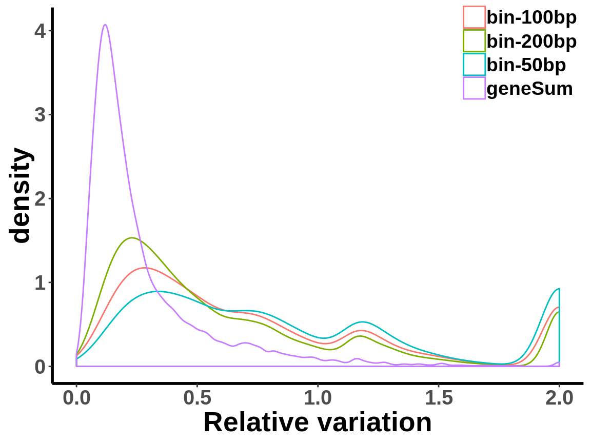

Compare MeRIP-seq IP data with regular RNA-seq data

var.coef <- function(x){sd(as.numeric(x))/mean(as.numeric(x))}

ip_coef_var <- t(apply(RADAR$ip_adjExpr_filtered,1,tapply,X,var.coef))
ip_coef_var <- ip_coef_var[!apply(ip_coef_var,1,function(x){return(any(is.na(x)))}),]
#hist(c(ip_coef_var),main = "M14KO mouse liver\n m6A-IP",xlab = "within group coefficient of variation",breaks = 50)
###
gene_coef_var <-  t(apply(RADAR$geneSum,1,tapply,X,var.coef))
gene_coef_var <- gene_coef_var[!apply(gene_coef_var,1,function(x){return(any(is.na(x)))}),]
#hist(c(gene_coef_var),main = "M14KO mouse liver\n RNA-seq",xlab = "within group coefficient of variation",breaks = 50)

coef_var <- list('RNA-seq'=c(gene_coef_var),'m6A-IP'=c(ip_coef_var))
nn<-sapply(coef_var, length)
rs<-cumsum(nn)
re<-rs-nn+1
grp <- factor(rep(names(coef_var), nn), levels=names(coef_var))
coef_var.df <- data.frame(coefficient_var = c(c(gene_coef_var),c(ip_coef_var)),label = grp)

ggplot(data = coef_var.df,aes(coefficient_var,colour = grp))+geom_density()+theme_bw() + theme(panel.border = element_blank(), panel.grid.major = element_blank(),
                   panel.grid.minor = element_blank(), axis.line = element_line(colour = "black",size = 1),
                   axis.title.x=element_text(size=20, face="bold", hjust=0.5,family = "arial"),
                   axis.title.y=element_text(size=20, face="bold", vjust=0.4, angle=90,family = "arial"),
                   legend.position = c(0.9,0.9),legend.title=element_blank(),legend.text = element_text(size = 18, face = "bold",family = "arial"),
                   axis.text.x = element_text(size = 15,face = "bold",family = "arial") ,axis.text.y = element_text(size = 15,face = "bold",family = "arial")  )+
  xlab("Coefficient of variation")

Check (within group) mean variance relationship of the data.

ip_var <- t(apply(RADAR$ip_adjExpr_filtered,1,tapply,RADAR$X,var))
#ip_var <- ip_coef_var[!apply(ip_var,1,function(x){return(any(is.na(x)))}),]
ip_mean <- t(apply(RADAR$ip_adjExpr_filtered,1,tapply,RADAR$X,mean))

###
gene_var <-  t(apply(RADAR$geneSum,1,tapply,X,var))
#gene_var <- gene_var[!apply(gene_var,1,function(x){return(any(is.na(x)))}),]
gene_mean <- t(apply(RADAR$geneSum,1,tapply,X,mean))

all_var <- list('RNA-seq'=c(gene_var),'m6A-IP'=c(ip_var))
nn<-sapply(all_var, length)
rs<-cumsum(nn)
re<-rs-nn+1
group <- factor(rep(names(all_var), nn), levels=names(all_var))
all_var.df <- data.frame(variance = c(c(gene_var),c(ip_var)),mean= c(c(gene_mean),c(ip_mean)),label = group)

ggplot(data = all_var.df,aes(x=mean,y=variance,colour = group,shape = group) )+geom_point(size = I(0.2))+stat_smooth(se = T,show.legend = F)+stat_smooth(se = F)+theme_bw() +xlab("Mean")+ ylab("Variance") + theme(panel.border = element_blank(), panel.grid.major = element_blank(),
                   panel.grid.minor = element_blank(), axis.line = element_line(colour = "black",size = 1),
                   axis.title.x=element_text(size=22, face="bold", hjust=0.5,family = "arial"),
                   axis.title.y=element_text(size=22, face="bold", vjust=0.4, angle=90,family = "arial"),
                   legend.position = c(0.85,0.95),legend.title=element_blank(),legend.text = element_text(size = 20, face = "bold",family = "arial"),
                   axis.text.x = element_text(size = 15,face = "bold",family = "arial") ,axis.text.y = element_text(size = 15,face = "bold",family = "arial")) +
  scale_x_continuous(limits = c(0,10000))+scale_y_continuous(limits = c(0,2.5e6),labels = scales::scientific)

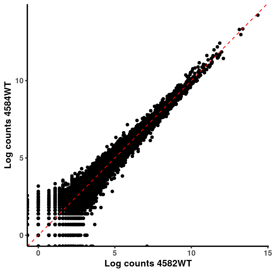
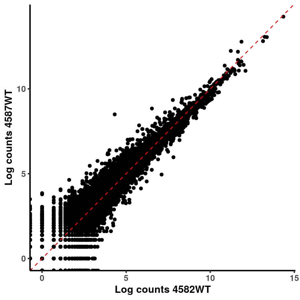
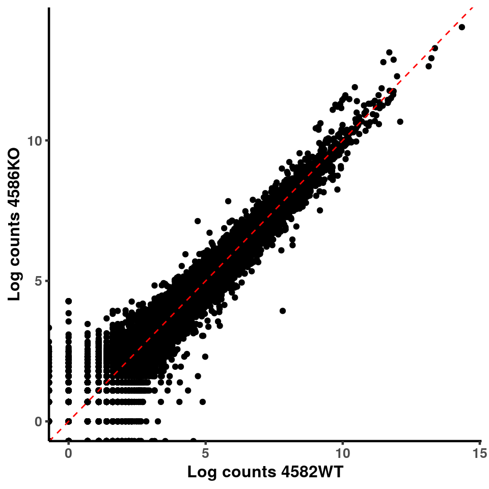
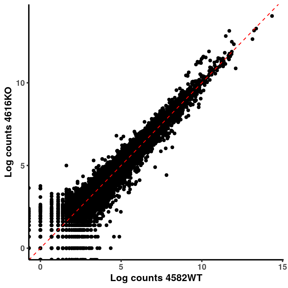
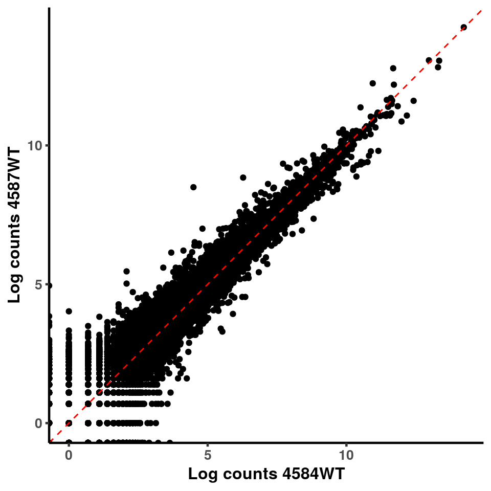
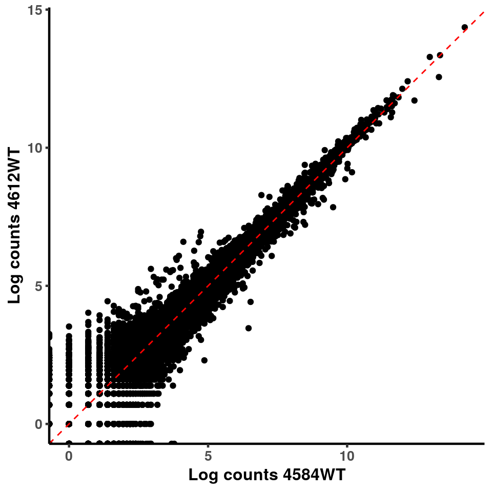
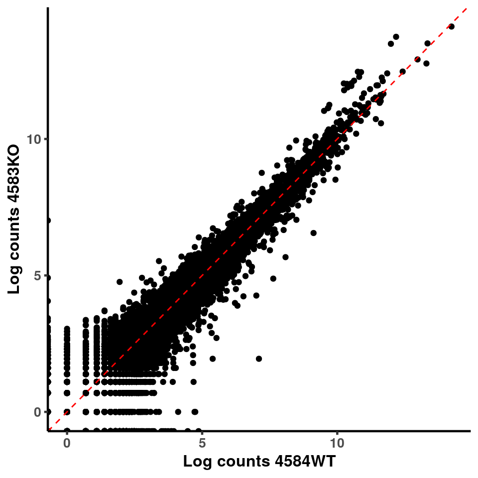
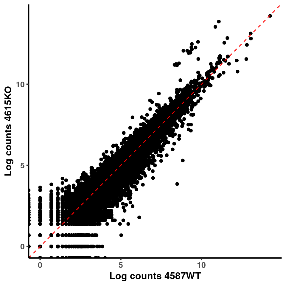
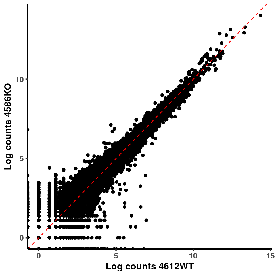
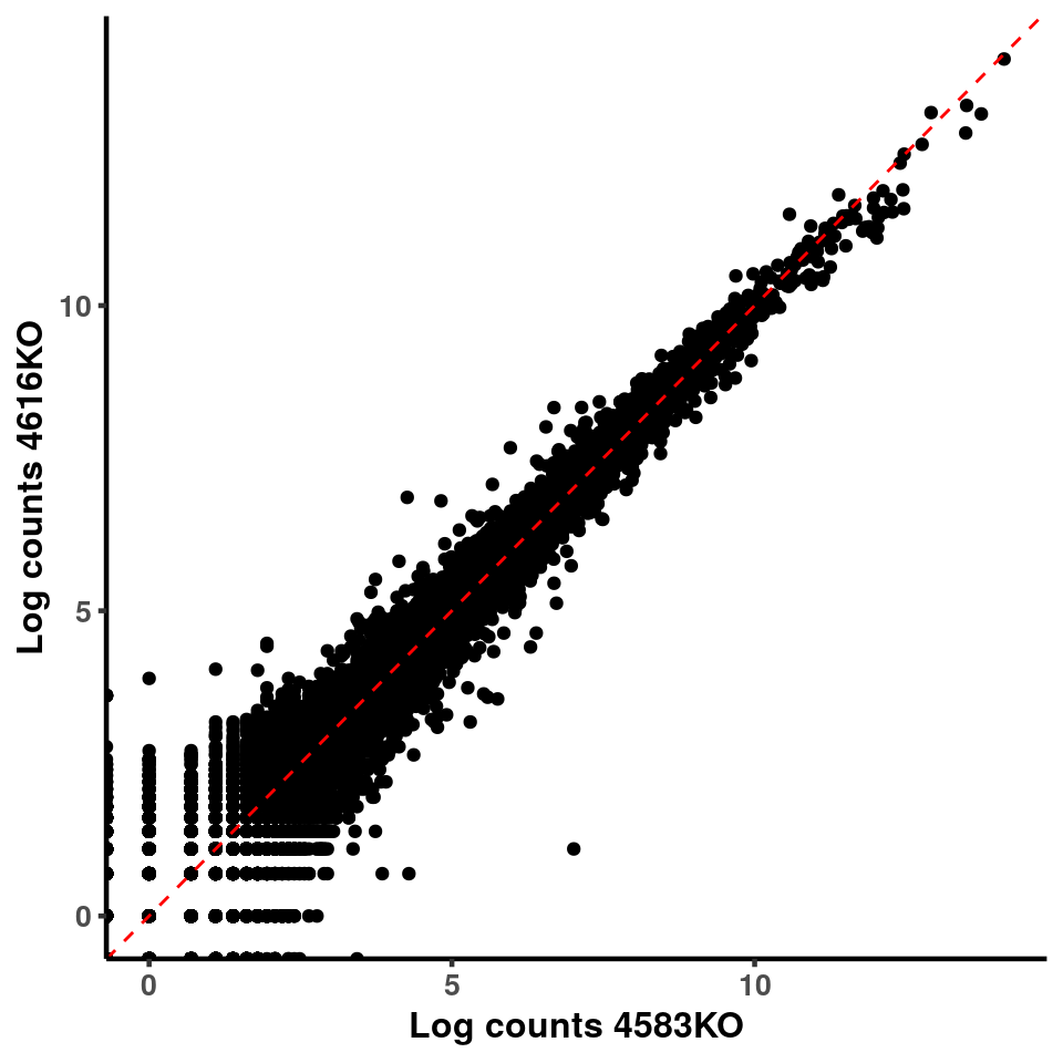
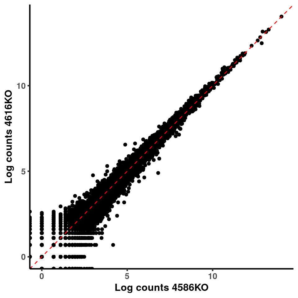
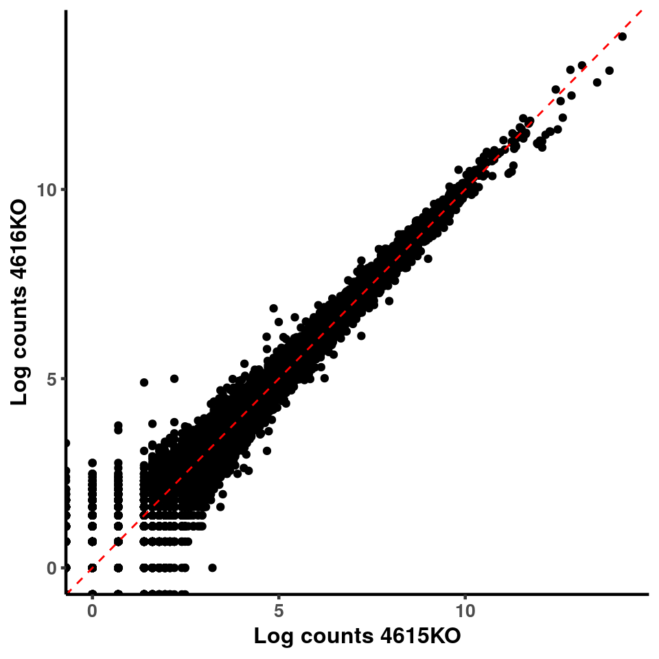
inputCount <- as.data.frame(RADAR$reads[,1:length(RADAR$samplenames)])
logInputCount <- as.data.frame(log( RADAR$geneSum  )  )
for(xx in 1:7){
  for(x in (xx+1):8){
  p <- ggplot(logInputCount, aes(x = logInputCount[,xx] , y = logInputCount[,x] ))+geom_point()+geom_abline(intercept = 0,slope = 1, lty = 2, colour = "red")+xlab(paste("Log counts",colnames(logInputCount)[xx],  sep = " ") )+ylab(paste("Log counts",colnames(logInputCount)[x],sep = " ") )+theme_classic(base_line_size = 0.8)+theme(axis.title = element_text(size = 12,face = "bold"), axis.text =  element_text(size = 10,face = "bold") )
  print(p)
  }
}

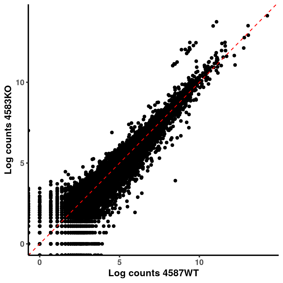
ggplot(logInputCount, aes(x = `4583KO` , y = `4587WT` ))+geom_point()+geom_abline(intercept = 0,slope = 1, lty = 2, colour = "red")+xlab(paste("Log counts 4583KO") )+ylab(paste("Log counts 4587WT") )+theme_classic(base_line_size = 0.8)+theme(axis.title = element_text(size = 12,face = "bold"), axis.text =  element_text(size = 10,face = "bold") )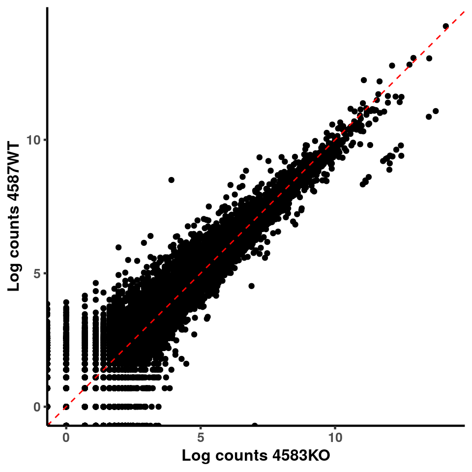

ggplot(logInputCount, aes(x = `4615KO` , y = `4584WT` ))+geom_point()+geom_abline(intercept = 0,slope = 1, lty = 2, colour = "red")+xlab(paste("Log counts 4615KO") )+ylab(paste("Log counts 4584WT") )+theme_classic(base_line_size = 0.8)+theme(axis.title = element_text(size = 12,face = "bold"), axis.text =  element_text(size = 10,face = "bold") )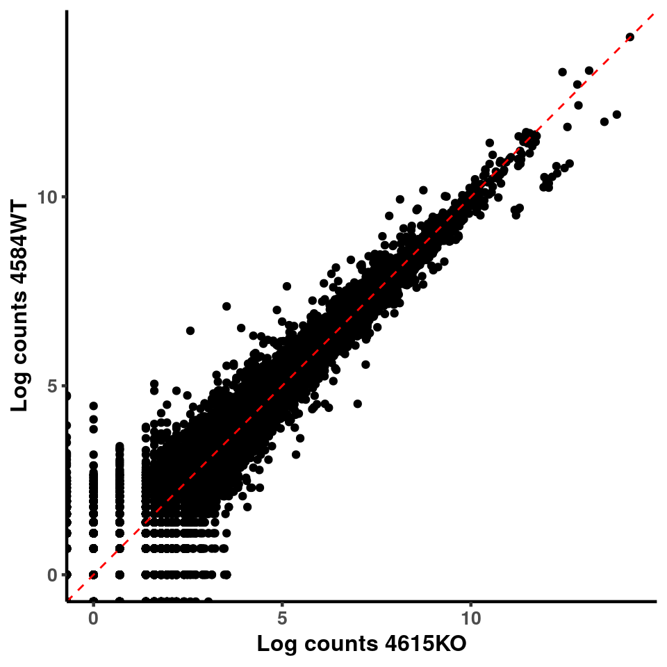

PCA analysis

After geting the filtered IP read count for testing, we can first use PCA analysis to check unkown variation.

top_bins <- RADAR$ip_adjExpr_filtered[order(rowMeans(RADAR$ip_adjExpr_filtered))[1:15000],]

We plot PCA colored by WT vs KO

plotPCAfromMatrix(top_bins,group = X)+scale_color_discrete(name = "Group")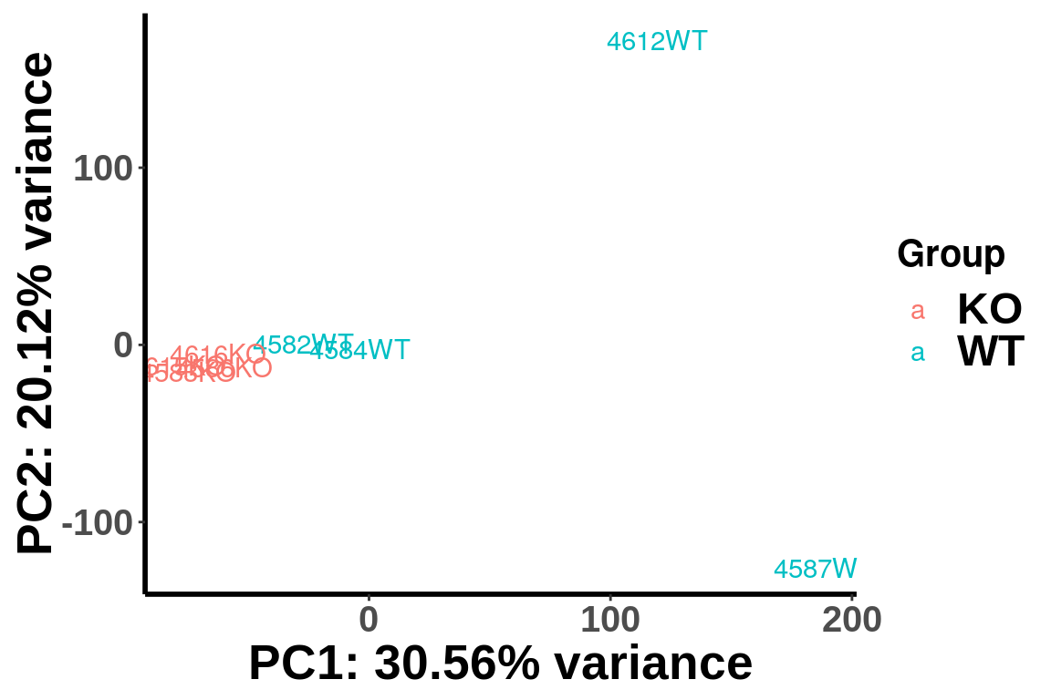

Run RADAR test

RADAR <- diffIP_parallel(RADAR)

Other method

In order to compare performance of other method on this data set, we run other three methods on default mode on this dataset.

deseq2.res <- DESeq2(countdata = RADAR$ip_adjExpr_filtered,pheno = matrix(c(rep(0,4),rep(1,4)),ncol = 1))
edgeR.res <- edgeR(countdata = RADAR$ip_adjExpr_filtered,pheno = matrix(c(rep(0,4),rep(1,4)),ncol = 1))

filteredBins <- rownames(RADAR$all.est)
QNB.res <- QNB::qnbtest(control_ip = RADAR$reads[filteredBins,9:12],
                        treated_ip = RADAR$reads[filteredBins,13:16],
                        control_input = RADAR$reads[filteredBins,1:4],
                        treated_input = RADAR$reads[filteredBins,5:8],plot.dispersion = FALSE)

Compare distribution of p value.

pvalues <- data.frame(pvalue = c(RADAR$all.est[,"p_value"],deseq2.res$pvalue,edgeR.res$pvalue,QNB.res$pvalue),
                      method = factor(rep(c("RADAR","DESeq2","edgeR","QNB"),c(length(RADAR$all.est[,"p_value"]),
                                                                       length(deseq2.res$pvalue),
                                                                       length(edgeR.res$pvalue),
                                                                       length(QNB.res$pvalue)
                                                                       )
                                          ),levels =c("RADAR","DESeq2","edgeR","QNB")
                                   )
                      )
ggplot(pvalues, aes(x = pvalue))+geom_histogram(breaks = seq(0,1,0.04),col=I("black"))+facet_grid(.~method)+theme_bw()+xlab("p-value")+theme( axis.title =  element_text(size = 22, face = "bold"),strip.text = element_text(size = 25, face = "bold"),axis.text.x = element_text(size = 18, face = "bold",colour = "black"),axis.text.y = element_text(size = 15, face = "bold",colour = "black",angle = 90),panel.grid = element_blank(), axis.line = element_line(size = 0.7 ,colour = "black"),axis.ticks = element_line(colour = "black"), panel.spacing = unit(0.4, "lines") )+ scale_x_continuous(breaks = seq(0,1,0.2),labels=function(x) sprintf("%.1f", x))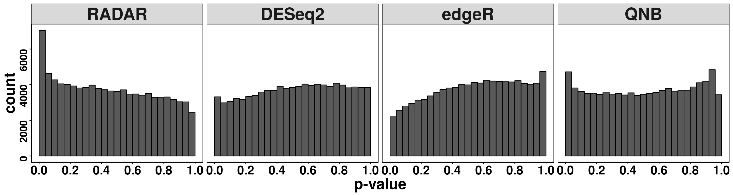

Compare the distibution of beta

par(mfrow = c(1,4))
hist(RADAR$all.est[,"beta"],main = "RADAR",xlab = "beta",breaks = 100,col =rgb(0.2,0.2,0.2,0.5),cex.main = 2.5,cex.axis =2,cex.lab=2)
hist(deseq2.res$log2FC, main = "DESeq2",xlab = "beta",breaks = 100,col =rgb(0.2,0.2,0.2,0.5),cex.main = 2.5,cex.axis =2,cex.lab=2)
hist(edgeR.res$log2FC,main = "edgeR", xlab = "beta",breaks = 100,col =rgb(0.2,0.2,0.2,0.5),cex.main = 2.5,cex.axis =2,cex.lab=2)
hist(QNB.res$log2.OR, main = "QNB",xlab = "beta",breaks = 100,col =rgb(0.2,0.2,0.2,0.5),cex.main = 2.5,cex.axis =2,cex.lab=2)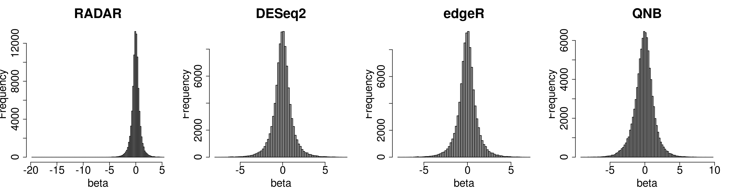

Plot overlap of significant hits

plot.new()
MyTools::venn_diagram3( names(which( qvalue::qvalue(RADAR$all.est[,"p_value"])$qvalue < 0.1 ) ),
                        rownames(RADAR$all.est)[which( qvalue::qvalue(deseq2.res$pvalue)$qvalue < 0.1 ) ],
                        rownames(RADAR$all.est)[which( qvalue::qvalue(QNB.res$pvalue)$qvalue < 0.1 ) ],
                        "RADAR","DESeq2","QNB")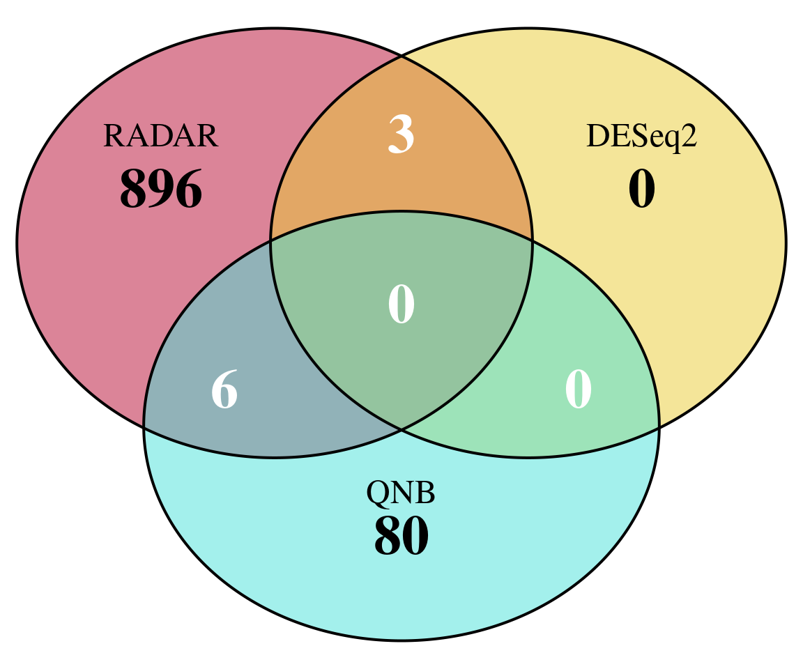

Session information

sessionInfo()

## R version 3.4.4 (2018-03-15)
## Platform: x86_64-pc-linux-gnu (64-bit)
## Running under: Ubuntu 17.10
##
## Matrix products: default
## BLAS: /usr/local/lib/R/lib/libRblas.so
## LAPACK: /usr/local/lib/R/lib/libRlapack.so
##
## locale:
##  [1] LC_CTYPE=en_US.UTF-8       LC_NUMERIC=C
##  [3] LC_TIME=en_US.UTF-8        LC_COLLATE=en_US.UTF-8
##  [5] LC_MONETARY=en_US.UTF-8    LC_MESSAGES=en_US.UTF-8
##  [7] LC_PAPER=en_US.UTF-8       LC_NAME=C
##  [9] LC_ADDRESS=C               LC_TELEPHONE=C
## [11] LC_MEASUREMENT=en_US.UTF-8 LC_IDENTIFICATION=C
##
## attached base packages:
##  [1] grid      stats4    parallel  stats     graphics  grDevices utils
##  [8] datasets  methods   base
##
## other attached packages:
##  [1] VennDiagram_1.6.20        futile.logger_1.4.3
##  [3] RADAR_0.1.5               RcppArmadillo_0.9.100.5.0
##  [5] Rcpp_0.12.19              RColorBrewer_1.1-2
##  [7] gplots_3.0.1              doParallel_1.0.14
##  [9] iterators_1.0.10          foreach_1.4.4
## [11] ggplot2_3.0.0             Rsamtools_1.30.0
## [13] Biostrings_2.46.0         XVector_0.18.0
## [15] GenomicFeatures_1.30.3    AnnotationDbi_1.40.0
## [17] Biobase_2.38.0            GenomicRanges_1.30.3
## [19] GenomeInfoDb_1.14.0       IRanges_2.12.0
## [21] S4Vectors_0.16.0          BiocGenerics_0.24.0
##
## loaded via a namespace (and not attached):
##  [1] nlme_3.1-131.1             bitops_1.0-6
##  [3] matrixStats_0.54.0         bit64_0.9-7
##  [5] progress_1.2.0             httr_1.3.1
##  [7] rprojroot_1.3-2            tools_3.4.4
##  [9] backports_1.1.2            R6_2.2.2
## [11] KernSmooth_2.23-15         mgcv_1.8-23
## [13] DBI_1.0.0                  lazyeval_0.2.1
## [15] colorspace_1.3-2           withr_2.1.2
## [17] tidyselect_0.2.4           gridExtra_2.3
## [19] prettyunits_1.0.2          RMySQL_0.10.15
## [21] bit_1.1-14                 compiler_3.4.4
## [23] formatR_1.5                DelayedArray_0.4.1
## [25] labeling_0.3               rtracklayer_1.38.3
## [27] caTools_1.17.1             scales_0.5.0
## [29] stringr_1.3.1              digest_0.6.15
## [31] rmarkdown_1.10             DOSE_3.4.0
## [33] pkgconfig_2.0.1            htmltools_0.3.6
## [35] highr_0.7                  rlang_0.2.1
## [37] RSQLite_2.1.1              bindr_0.1.1
## [39] BiocParallel_1.12.0        gtools_3.8.1
## [41] GOSemSim_2.4.1             dplyr_0.7.6
## [43] RCurl_1.95-4.10            magrittr_1.5
## [45] GO.db_3.5.0                GenomeInfoDbData_1.0.0
## [47] Matrix_1.2-12              munsell_0.5.0
## [49] stringi_1.2.3              yaml_2.1.19
## [51] SummarizedExperiment_1.8.1 zlibbioc_1.24.0
## [53] plyr_1.8.4                 qvalue_2.10.0
## [55] blob_1.1.1                 gdata_2.18.0
## [57] DO.db_2.9                  crayon_1.3.4
## [59] lattice_0.20-35            splines_3.4.4
## [61] hms_0.4.2                  knitr_1.20
## [63] pillar_1.2.3               fgsea_1.4.1
## [65] igraph_1.2.1               reshape2_1.4.3
## [67] codetools_0.2-15           biomaRt_2.34.2
## [69] futile.options_1.0.1       fastmatch_1.1-0
## [71] XML_3.98-1.11              glue_1.2.0
## [73] evaluate_0.10.1            lambda.r_1.2.3
## [75] data.table_1.11.4          tidyr_0.8.1
## [77] gtable_0.2.0               purrr_0.2.5
## [79] assertthat_0.2.0           tibble_1.4.2
## [81] clusterProfiler_3.6.0      rvcheck_0.1.0
## [83] GenomicAlignments_1.14.2   memoise_1.1.0
## [85] MyTools_0.0.0              bindrcpp_0.2.2

This R Markdown site was created with workflowr